Plot the treated and control outcome fits from a causal model
plot.mixgpd_fit.Rdplot.causalmixgpd_causal_fit() is a convenience router to the
underlying one-arm diagnostic plots for the treated and control fits.
Uses ggmcmc to produce standard MCMC diagnostic plots. Works with 1+ chains.
S3 method for visualizing fitted values from fitted.mixgpd_fit().
Produces a 2-panel figure: Q-Q plot and residuals vs fitted.
Arguments
- x
Object of class
mixgpd_fittedfromfitted.mixgpd_fit().- arm
Integer or character;
1or"treated"for treatment,0or"control"for control, or"both"for both arms.- ...
Additional arguments (ignored).
- family
Character vector of plot names (ggmcmc plot types) or a single one. The default
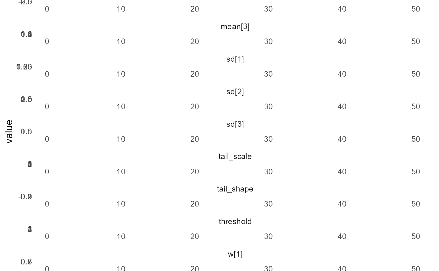
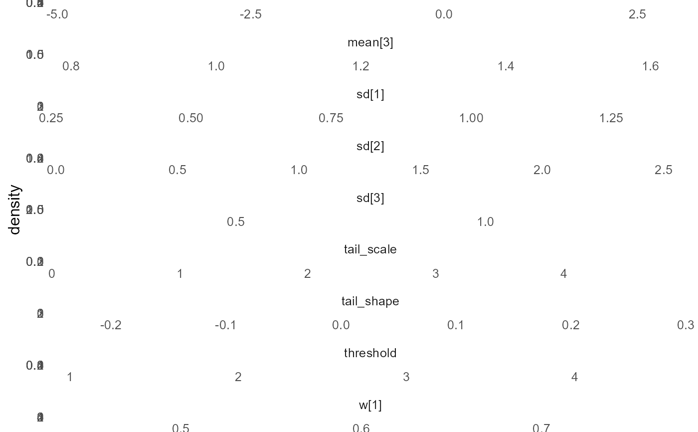
"traceplot"returns one diagnostic. Use"all"to include all plots supported for the available number of chains/parameters."auto"is accepted as an alias for the default single diagnostic. Supported types:"histogram": posterior histograms"density": posterior density curves"traceplot": MCMC trace plots"running": running mean plots"compare_partial": partial chain comparisons"autocorrelation": autocorrelation plots"crosscorrelation": cross-correlation matrix"Rhat": Gelman–Rubin R-hat (2+ chains)"grb": Gelman–Rubin–Brooks (2+ chains)"effective": effective sample size"geweke": Geweke diagnostic"caterpillar": caterpillar/forest plots"pairs": pairwise scatter plots (2+ params)
- params
Optional parameter selector:
character vector of parameter patterns (exact names or partial matches)
a single regex string (e.g.
"alpha|threshold|tail_")NULL(default): plots all monitored parameters
- nLags
Number of lags for autocorrelation (ggmcmc).
- y
Ignored; included for S3 compatibility.
Value
The result of the underlying plot call (invisibly).
Invisibly returns a named list of ggplot objects.
Invisibly returns a list with the two plots.
Details
Each arm-specific outcome model is itself a mixgpd_fit, so this method
delegates to plot.mixgpd_fit() for the selected arm. With arm = "both",
it returns a named list of treated and control diagnostics so the two fitted
outcome models can be assessed side by side.
These are MCMC diagnostics for the nuisance outcome models, not plots of
causal estimands. Use plot() on objects from
predict.causalmixgpd_causal_fit(), qte(), or ate() when the goal is to
visualize treatment effects rather than chain behavior.
The supported plots diagnose posterior simulation quality rather than data fit.
Depending on the selected family, they show chain traces, marginal posterior
densities, autocorrelation, cross-correlation, running means, or Gelman-style
convergence summaries for the monitored parameters.
These graphics should be read before interpreting posterior summaries or treatment-effect results. Poor mixing or strong autocorrelation in the MCMC output can invalidate downstream summaries even when the fitted model itself is correctly specified.
These diagnostics compare the fitted values implied by the posterior summary on the training design against the observed responses. The first panel checks how closely fitted and observed values align, while the second panel looks for residual structure that would indicate lack of fit or remaining mean trends.
This method is distinct from posterior predictive simulation on new data. It
is a training-sample diagnostic built from fitted.mixgpd_fit() and the
corresponding residuals.
See also
plot.mixgpd_fit,
predict.causalmixgpd_causal_fit, ate,
qte.
Examples
# \donttest{
y <- abs(stats::rnorm(25)) + 0.1
bundle <- build_nimble_bundle(y = y, backend = "sb", kernel = "normal",
GPD = TRUE, components = 3,
mcmc = list(niter = 100, nburnin = 50, thin = 1, nchains = 1))
fit <- run_mcmc_bundle_manual(bundle)
#> [mixgpd] Validating configuration
#> [mixgpd] Checking build/compile cache
#> [mixgpd] Building model and MCMC configuration
#> [mixgpd] Compiling NIMBLE model
#> [mixgpd] Initializing chains
#> [mixgpd] Running MCMC
#> [mixgpd] Finalizing WAIC and diagnostics
#> [mixgpd] Assembling fit object
plot(fit, family = c("traceplot", "density"))
#> Scale for colour is already present.
#> Adding another scale for colour, which will replace the existing scale.
#> Scale for colour is already present.
#> Adding another scale for colour, which will replace the existing scale.
#>
#> === traceplot ===
 #>
#> === density ===
#>
#> === density ===
 # }
# }