Advanced: GPD-in-DPM architecture (CRP-only)

Advanced user vignette. CRP-only prototype for a Dirichlet process mixture in which the cluster atom is a scalar kernel parameter and the observation model uses the exported GPD-spliced kernel distributions.

Keywords

advanced, CRP, DPM, GPD, nimble

Advanced users only

This vignette is a code-oriented prototype. It assumes familiarity with NIMBLE model code and with validating custom Bayesian nonparametric models.

1 Objective

The package currently provides bulk-only mixtures (d*Mix) and bulk-tail spliced distributions (d*Gpd, d*MixGpd) as NIMBLE nimbleFunctions. However, it does not yet expose a “scalar-atom DPM with an embedded GPD tail” as a one-line high-level interface.

For the formal bulk-vs-tail splicing definitions (threshold exceedances, GPD tail quantiles, and spliced CDF/density), see Theory: GPD tails + DPM bulk + splicing.

The goal here is to show how to write that model directly in nimbleCode{} for the CRP backend, while reusing the exported spliced distributions (e.g., dGammaGpd, dLognormalGpd, dInvGaussGpd, dNormGpd, etc.). No ones/zeros trick is required because the likelihood is written using these distributions directly.

2 Model specification

Let (y_1,,y_N) be observations. Under a CRP DPM:

Latent cluster labels follow a Chinese restaurant process: [ z[1{:}N] (), ] implemented in NIMBLE as z[1:N] ~ dCRP(conc = alpha, size = N).
Each cluster (k) has a scalar atom (_k). The atom is the only cluster-specific kernel parameter; all other kernel parameters are fixed or global.
Conditional on the latent cluster label, the observation likelihood uses a GPD-spliced kernel distribution exported by the package. For a positive-support outcome, a convenient choice is Gamma+GPD: [ y_i z_i=k (=a, =k, u, {}, ), ] where the Gamma is used below the threshold (u), and exceedances use the GPD tail via dGpd inside dGammaGpd.

This construction is “GPD-in-DPM” in the sense that the tail is part of the per-observation distribution (not a separate post-processing step), while the mixture is induced by the CRP cluster labels.

3 A concrete working template (Gamma bulk, scalar scale atom)

The template below uses:

scalar atom: scale_k = theta[k] > 0
fixed bulk shape: shape0 (constant)
tail parameters: threshold, tail_scale, tail_shape (constants or global parameters)

You can substitute a different exported spliced distribution by changing the likelihood line (for example, dLognormalGpd, dInvGaussGpd, dNormGpd, etc.).

Code

library(CausalMixGPD)
library(nimble)

# Data shipped with the package (positive-support, tail-designed)
data("nc_pos_tail200_k4")
y <- nc_pos_tail200_k4$y
N <- length(y)

# Use the dataset's generating tail settings (keeps the example coherent)
threshold  <- nc_pos_tail200_k4$truth$threshold
tail_scale <- nc_pos_tail200_k4$truth$tail_params$scale
tail_shape <- nc_pos_tail200_k4$truth$tail_params$shape


# Choose a truncation level for the finite representation of clusters
components <- 25

# Fixed bulk shape (example)
shape0 <- 2.0


code <- nimbleCode({
  # Concentration
  alpha ~ dgamma(1, 1)

  # Scalar atoms (cluster-specific). Here: positive scale parameters.
  for (k in 1:components) {
    theta[k] ~ dgamma(a0, b0)
  }

  # CRP memberships (native NIMBLE BNP distribution)
  z[1:N] ~ dCRP(conc = alpha, size = N)

  # Likelihood: exported spliced kernel distribution
  for (i in 1:N) {
    y[i] ~ dGammaGpd(shape = shape0,
                     scale = theta[z[i]],
                     threshold = threshold,
                     tail_scale = tail_scale,
                     tail_shape = tail_shape)
  }
})

constants <- list(
  N = N, components = components,
  a0 = 2, b0 = 2,
  shape0 = shape0,
  threshold = threshold,
  tail_scale = tail_scale,
  tail_shape = tail_shape
)

data <- list(y = y)

inits <- list(
  alpha = 1,
  theta = rgamma(components, 2, 2),
  z = sample.int(5, N, replace = TRUE)
)

m <- nimbleModel(code, constants = constants, data = data, inits = inits, check = TRUE)
cm <- compileNimble(m)

conf <- configureMCMC(m, monitors = c("alpha", "theta", "z"))

===== Monitors =====
thin = 1: alpha, theta, z
===== Samplers =====
CRP_concentration sampler (1)
  - alpha
CRP_cluster_wrapper sampler (25)
  - theta[]  (25 elements)
CRP sampler (1)
  - z[1:200]

Code

mcmc <- buildMCMC(conf)
cmcmc <- compileNimble(mcmc, project = m)

samps <- runMCMC(cmcmc, niter = 600, nburnin = 300, thin = 2, setSeed = 1)

|-------------|-------------|-------------|-------------|
|-------------------------------------------------------|

4 Posterior analysis

This section sketches a minimal posterior workflow after runMCMC() returns samps. The object returned by runMCMC() is typically a matrix with one row per retained iteration and one column per monitored node.

4.1 Basic parameter summaries

Code

# Posterior summary for alpha
alpha_draws <- samps[, "alpha"]
summary(alpha_draws)

   Min. 1st Qu.  Median    Mean 3rd Qu.    Max. 
0.06258 0.43053 0.71488 0.85106 1.05312 4.22596

Code

# Posterior summaries for the scalar atoms theta[k]
theta_cols  <- grep("^theta\\[", colnames(samps), value = TRUE)
theta_draws <- samps[, theta_cols, drop = FALSE]

theta_summary <- t(apply(theta_draws, 2, function(x) {
  c(mean = mean(x), sd = sd(x),
    q025 = unname(quantile(x, 0.025)),
    q50  = unname(quantile(x, 0.50)),
    q975 = unname(quantile(x, 0.975)))
}))

kableExtra::kbl(theta_summary, digits = 3, caption = "Posterior summaries of scalar atoms (theta[k])") |>
  kableExtra::kable_styling(full_width = FALSE)

Posterior summaries of scalar atoms (theta[k])
	mean	sd	q025	q50	q975
theta[1]	0.991	0.622	0.333	0.806	2.593
theta[2]	1.180	0.796	0.339	0.951	2.846
theta[3]	1.379	0.467	0.812	1.208	2.356
theta[4]	1.038	0.540	0.182	0.956	2.265
theta[5]	1.025	0.483	0.394	0.862	2.446
theta[6]	1.157	0.725	0.249	0.992	2.869
theta[7]	1.216	0.575	0.291	1.085	2.447
theta[8]	1.790	1.069	0.197	2.496	2.794
theta[9]	0.584	0.770	0.300	0.341	3.512
theta[10]	0.713	0.121	0.664	0.707	0.922
theta[11]	0.882	0.297	0.611	0.793	1.683
theta[12]	1.744	0.659	0.744	2.324	2.324
theta[13]	0.870	0.546	0.287	1.086	2.096
theta[14]	0.700	0.121	0.383	0.637	0.827
theta[15]	0.964	0.277	0.725	0.725	1.261
theta[16]	1.109	0.000	1.109	1.109	1.109
theta[17]	0.131	0.000	0.131	0.131	0.131
theta[18]	1.090	0.000	1.090	1.090	1.090
theta[19]	0.954	0.000	0.954	0.954	0.954
theta[20]	0.536	0.000	0.536	0.536	0.536
theta[21]	1.013	0.000	1.013	1.013	1.013
theta[22]	0.981	0.000	0.981	0.981	0.981
theta[23]	2.387	0.000	2.387	2.387	2.387
theta[24]	1.289	0.000	1.289	1.289	1.289
theta[25]	0.820	0.000	0.820	0.820	0.820

4.2 Posterior clustering diagnostics

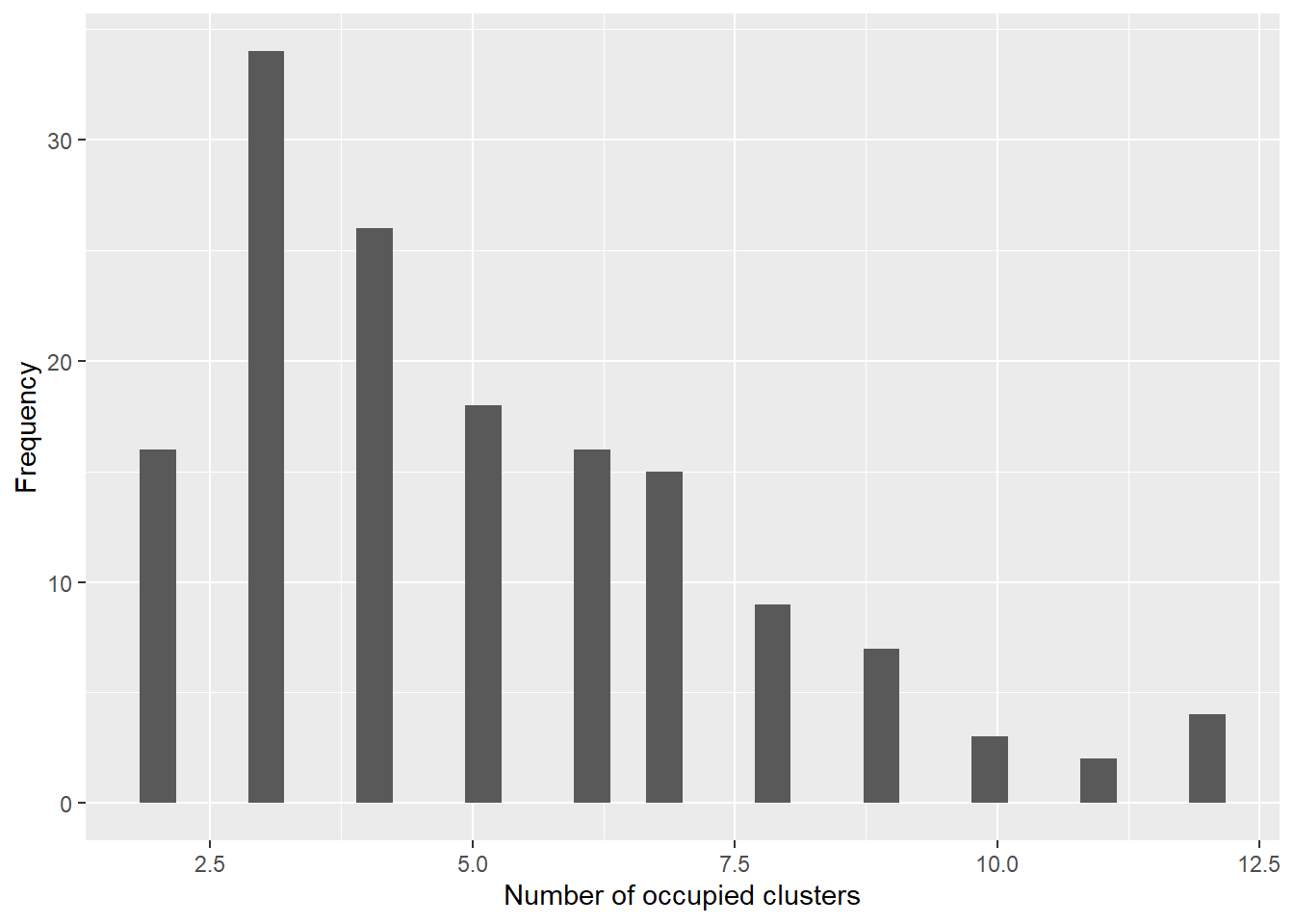
A practical summary of the induced partition is the posterior distribution of the number of occupied clusters, [ K^{(m)} = |{ z^{(m)}_1,,z^{(m)}_N }|, ] computed for each retained iteration (m).

Code

z_cols  <- grep("^z\\[", colnames(samps), value = TRUE)
z_draws <- samps[, z_cols, drop = FALSE]

K_occ <- apply(z_draws, 1, function(zrow) length(unique(as.integer(zrow))))

summary(K_occ)

   Min. 1st Qu.  Median    Mean 3rd Qu.    Max. 
  2.000   3.000   4.000   5.093   7.000  12.000

Code

dfK <- data.frame(K = K_occ)
ggplot2::ggplot(dfK, ggplot2::aes(x = K)) +
  ggplot2::geom_histogram(bins = 30) +
  ggplot2::labs(x = "Number of occupied clusters", y = "Frequency")

If you monitor z, this can be memory-heavy for large (N). For posterior diagnostics only, consider monitoring z for a subsample of observations, or derive K_occ inside NIMBLE using deterministic nodes (advanced).

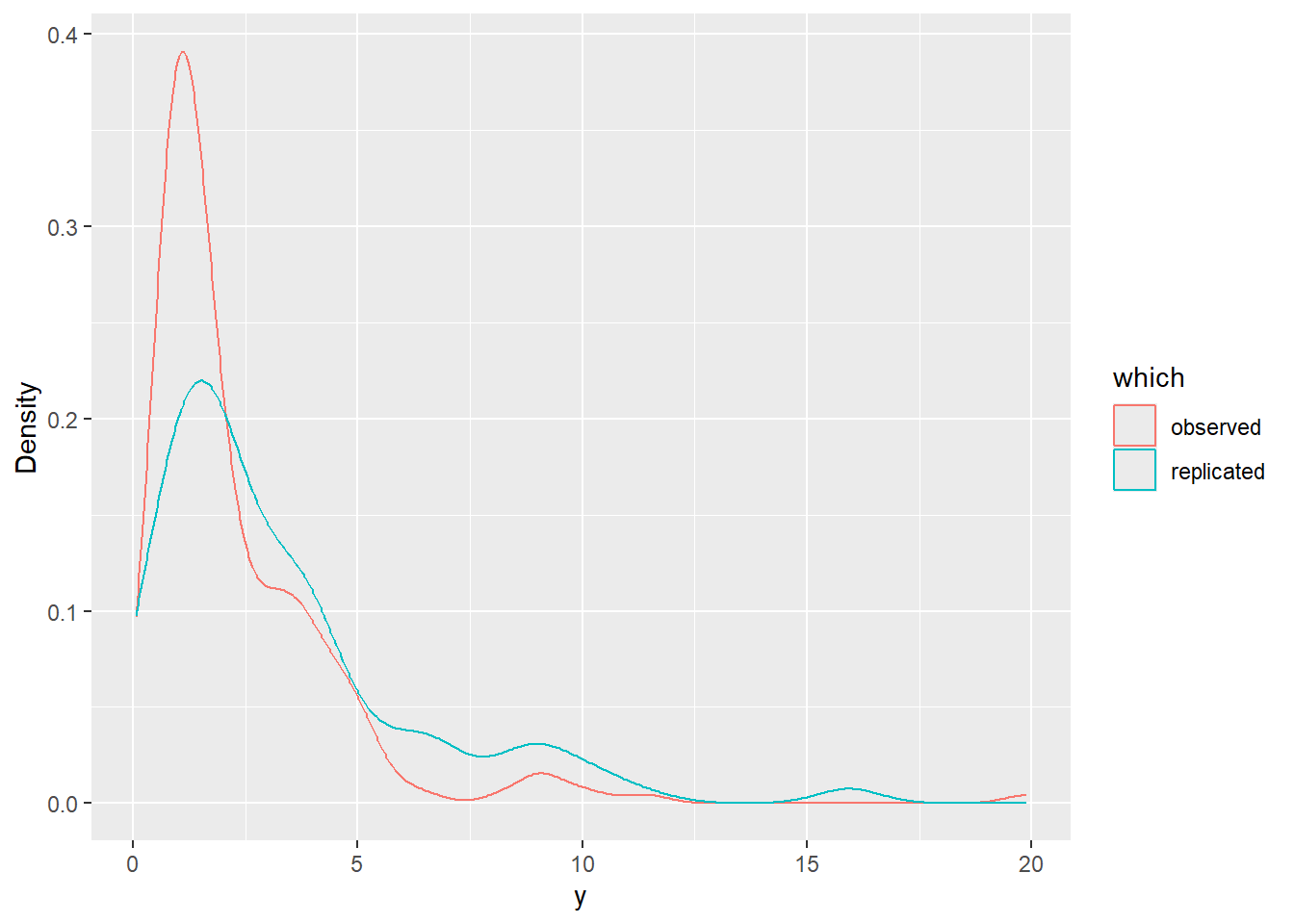
4.3 Posterior predictive checks

A simple posterior predictive check is to generate replicated outcomes (y^{rep}) from the fitted model and compare distributional features.

For the CRP mixture, one convenient approximation is to sample a cluster label for a new observation using empirical cluster frequencies from the current iteration (ignoring the “new cluster” probability). This yields a practical in-sample predictive check and is typically sufficient for early debugging.

Code

# Extract theta and z at each iteration
theta_mat <- theta_draws
z_mat     <- z_draws

# One posterior predictive draw per iteration (increase B if needed)
M <- nrow(samps)
y_rep <- numeric(M)

for (m in 1:M) {
  z_m <- as.integer(z_mat[m, ])
  # empirical cluster weights
  tab <- table(z_m)
  labs <- as.integer(names(tab))
  w <- as.numeric(tab) / sum(tab)

  k_new <- sample(labs, size = 1, prob = w)
  scale_new <- theta_mat[m, sprintf("theta[%d]", k_new)]

  y_rep[m] <- rGammaGpd(
    1,
    shape = shape0,
    scale = scale_new,
    threshold = threshold,
    tail_scale = tail_scale,
    tail_shape = tail_shape
  )
}

# Compare observed vs replicated summaries
quantile(y, probs = c(0.5, 0.9, 0.95, 0.99))

      50%       90%       95%       99% 
 1.522206  4.596914  5.318649 10.261557

Code

quantile(y_rep, probs = c(0.5, 0.9, 0.95, 0.99))

      50%       90%       95%       99% 
 2.351143  7.993032  9.390843 13.751122

Code

dfppc <- data.frame(value = c(y, y_rep),
                    which = rep(c("observed", "replicated"), c(length(y), length(y_rep))))

ggplot2::ggplot(dfppc, ggplot2::aes(x = value, colour = which)) +
  ggplot2::geom_density() +
  ggplot2::labs(x = "y", y = "Density")

4.4 Tail summaries from the posterior

Two basic tail summaries are:

exceedance probability ( (Y > u) ),
extreme quantiles (e.g., (q_{0.99})).

With posterior predictive draws y_rep, you can estimate both directly:

Code

mean(y_rep > threshold)                      # posterior predictive exceedance rate

[1] 0.4

Code

quantile(y_rep, probs = c(0.95, 0.99, 0.995))

      95%       99%     99.5% 
 9.390843 13.751122 15.915371

For more precise quantiles (and to reduce Monte Carlo error), increase the number of predictive draws per iteration or compute the predictive CDF as a mixture of p*Gpd terms and solve for the quantile (more expensive; recommended only after the baseline model is stable).

5 How to adapt this template

Select the appropriate spliced distribution for the support of your outcome:

Positive support: dGammaGpd, dLognormalGpd, dInvGaussGpd, dAmorosoGpd, etc.
Real line: dNormGpd or a suitable real-line kernel if available.

Identify a single kernel parameter to serve as the scalar atom (_k), and fix or globalize the remaining kernel parameters.
Decide whether threshold, tail_scale, and tail_shape are fixed constants, global parameters with priors, or covariate-linked (the last option is more involved and should be introduced only after the baseline model is stable).

6 Minimal validation requirements

Before applying the model to real data:

Perform simulation recovery under the same kernel and tail settings.
Check posterior predictive exceedance rates above threshold.
Check sensitivity to the chosen threshold and priors on alpha and tail parameters.

6.1 Prereqs

Required packages and data for this page are listed in the setup chunks above.

6.2 Outputs

This page renders model fits, diagnostics, and summary artifacts generated by package APIs.

6.3 Interpretation

Canonical concept page: 01 Gpd Dp Setup
Treat this page as an application/example view and use the canonical page for core definitions.

6.4 Next

Continue to the linked canonical concept page, then return for implementation-specific details.