Plot prediction results — plot.mixgpd

Generates type-specific visualizations for prediction objects returned by predict.mixgpd_fit(). Each prediction type produces a tailored plot:

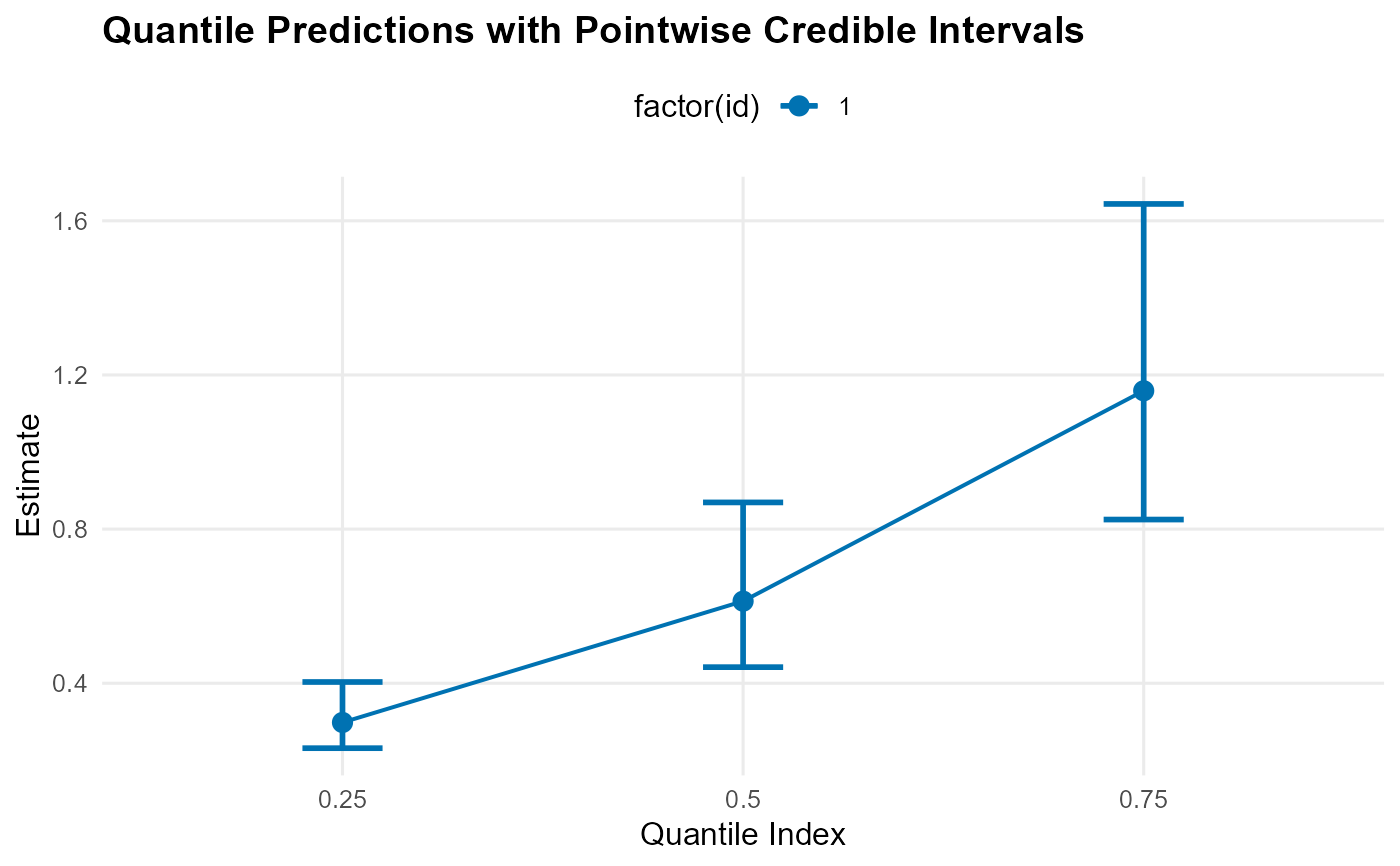
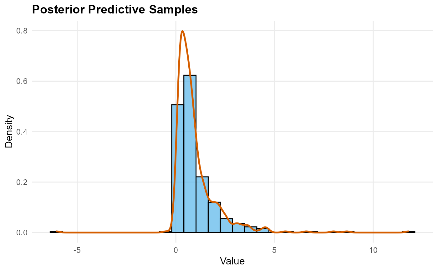
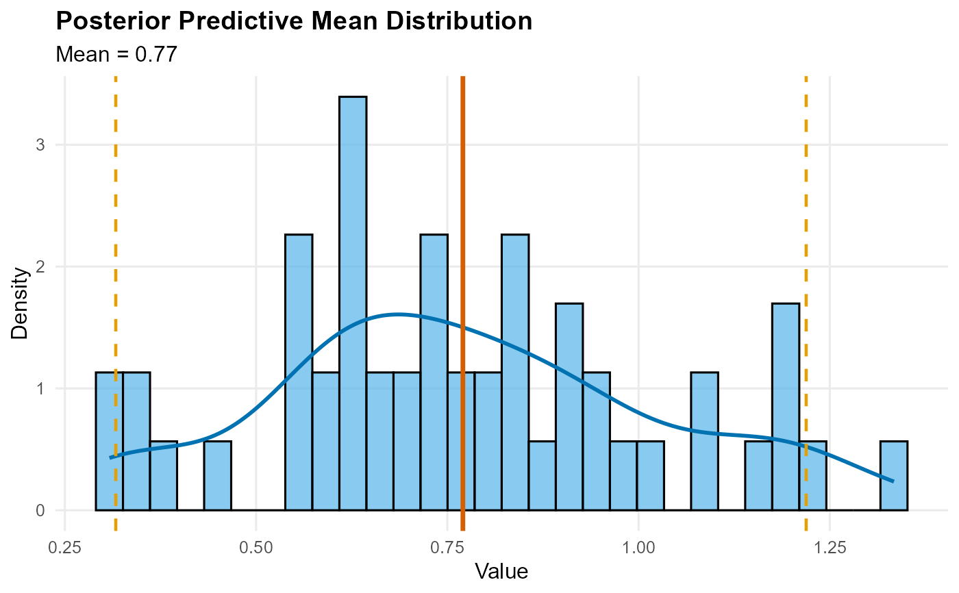
quantile: Quantile indices vs estimates with credible intervals
sample: Histogram of samples with density overlay
mean: Histogram density with posterior mean vertical line and CI bounds
density: Density values vs evaluation points
survival: Survival function (decreasing y values)

S3 method for visualizing causal predictions from predict.causalmixgpd_causal_fit(). For mean/quantile, plots treated/control and treatment effect versus PS (or index). For type = "sample", plots arm-level posterior predictive samples alongside treatment-effect samples. For density/prob, plots treated/control values versus y.

Usage

# S3 method for class 'mixgpd_predict'
plot(x, y = NULL, ...)

# S3 method for class 'causalmixgpd_causal_predict'
plot(x, y = NULL, ...)

Arguments

x: Object of class causalmixgpd_causal_predict.
y: Ignored.
...: Additional arguments passed to ggplot2 functions.

Value

Invisibly returns the ggplot object.

A ggplot object or a list of ggplot objects.

Details

The plotting method is tied to the predictive functional stored in the input object. Quantile and mean outputs display posterior point summaries and intervals, density and survival outputs show evaluated functions on the supplied grid, and posterior samples are visualized as empirical predictive draws.

In every case the plot reflects the quantity requested from predict.mixgpd_fit() after integrating over the retained posterior draws. It is therefore distinct from parameter-level summaries and from chain diagnostics.

The causal prediction object carries arm-specific predictions together with the implied contrast. For mean predictions, the contrast is \(m_1(x) - m_0(x)\). For quantile predictions, the contrast is \(Q_{Y^1}(\tau \mid x) - Q_{Y^0}(\tau \mid x)\). The plotting method keeps those arm and contrast views synchronized.

Unlike plot.causalmixgpd_causal_fit(), which diagnoses MCMC behavior inside the outcome models, this method visualizes predictive quantities after posterior integration. It is therefore the natural plotting method once the user has already accepted the fitted-model diagnostics.

Examples

# \donttest{
y <- abs(stats::rnorm(25)) + 0.1
bundle <- build_nimble_bundle(y = y, backend = "sb", kernel = "normal",
                             GPD = TRUE, components = 3,
                             mcmc = list(niter = 100, nburnin = 50, thin = 1, nchains = 1))
fit <- run_mcmc_bundle_manual(bundle)
#> [mixgpd] Validating configuration
#> [mixgpd] Checking build/compile cache
#> [mixgpd] Building model and MCMC configuration
#> [mixgpd] Compiling NIMBLE model
#> [mixgpd] Initializing chains
#> [mixgpd] Running MCMC
#> [mixgpd] Finalizing WAIC and diagnostics
#> [mixgpd] Assembling fit object

# Quantile prediction with plot
pred_q <- predict(fit, type = "quantile", index = c(0.25, 0.5, 0.75))
#> [predict_mixgpd] Validating prediction inputs
#> [predict_mixgpd] Extracting posterior draws
#> [predict_mixgpd] Computing posterior summaries
#> [predict_mixgpd] Assembling prediction output
plot(pred_q)


# Sample prediction with plot
pred_s <- predict(fit, type = "sample", nsim = 500)
#> [predict_mixgpd] Validating prediction inputs
#> [predict_mixgpd] Extracting posterior draws
#> [predict_mixgpd] Computing posterior summaries
#> [predict_mixgpd] Assembling prediction output
plot(pred_s)


# Mean prediction with plot
pred_m <- predict(fit, type = "mean", nsim_mean = 300)
#> [predict_mixgpd] Validating prediction inputs
#> [predict_mixgpd] Extracting posterior draws
#> [predict_mixgpd] Computing posterior summaries
#> [predict_mixgpd] Assembling prediction output
plot(pred_m)

# }