Advanced: Customization and tuning

Overview

This vignette documents how to construct and run NIMBLE models using the low-level building blocks exported by CausalMixGPD. The intended audience is advanced users who want full control of the model specification while still reusing the package’s NIMBLE-ready distributions (mixture kernels and bulk-tail splices) and the standard NIMBLE compilation and MCMC workflow.

The examples emphasize transparency. Each model is specified in nimbleCode{}; constants, data, and initial values are stated explicitly; and the model is compiled and sampled using the canonical NIMBLE sequence.

The vignette covers:

For the underlying “where each option lives” map (core customization surface + extension points), see Theory: Customization maps + extension points.

A manual stick-breaking (SB) Normal mixture using dNormMix as the likelihood.
A spliced bulk-tail model (SB + Amoroso + GPD) in which CausalMixGPD generates the model code, while the compilation and sampling steps are carried out explicitly to facilitate inspection.
A causal (two-arm) model built via bundle(), followed by downstream summaries via S3 methods such as predict(), ate()/qte() (marginal), att()/qtt() (treated-only), and cate()/cqte() (conditional; requires X).

Throughout, the focus is on reproducible model construction and on using the exported NIMBLE distributions directly in the likelihood. In this setting, a ones/zeros trick is not required.

Data

Code

data("mtcars", package = "datasets")

df <- mtcars
y <- df$mpg
X <- df[, c("wt", "hp")]
X <- as.data.frame(X)

SB Case: Manual Stick-Breaking Model with `dNormMix`

In this first example we write an SB mixture model by hand and use the exported dNormMix() nimbleFunction as the per-observation log-likelihood. The point is to show that CausalMixGPD kernels are ordinary NIMBLE components: you can call them inside your own model code, monitor whatever nodes you like, and control the MCMC configuration exactly as you would in a standalone NIMBLE workflow.

Note on custom likelihoods

NIMBLE can work with user-defined distributions, but for a vignette it is often easier to avoid registration and keep everything “plain” model code. CausalMixGPD already exposes the mixture and MixGPD building blocks as NIMBLE distributions (e.g., dNormMix for a Normal mixture and dNormMixGpd for the spliced bulk+GPD version). That means you can write the likelihood directly in nimbleCode using y[i] ~ dNormMix(...) or y[i] ~ dNormMixGpd(...)–no ones/zeros trick is needed here.

Constants, data, and inits

Code

N <- length(y)
K <- 3

constants_sb <- list(N = N, K = K)
data_sb <- list(y = y)

inits_sb <- function() {
  list(
    alpha = 1,
    v = c(rep(0.5, K - 1), 1),
    mu = rnorm(K, mean(y), 1),
    sigma = rep(sd(y), K)
  )
}

NIMBLE code

Code

code_sb <- nimble::nimbleCode({
  alpha ~ dgamma(1, 1)

  for (k in 1:(K - 1)) {
    v[k] ~ dbeta(1, alpha)
  }
  v[K] <- 1

  w[1] <- v[1]
  for (k in 2:K) {
    w[k] <- v[k] * prod(1 - v[1:(k - 1)])
  }

  for (k in 1:K) {
    mu[k] ~ dnorm(0, sd = 5)
    sigma[k] ~ dunif(0.1, 5)
  }

  for (i in 1:N) {
    y[i] ~ dNormMix(w = w[1:K], mean = mu[1:K], sd = sigma[1:K])
  }
})

Compile and run (manual)

Code

. <- utils::capture.output({
  Rmodel_sb <- nimble::nimbleModel(
    code = code_sb,
    constants = constants_sb,
    data = data_sb,
    inits = inits_sb()
  )

  conf_sb <- nimble::configureMCMC(
    Rmodel_sb,
    monitors = c("alpha", "v", "w", "mu", "sigma")
  )

  Rmcmc_sb <- nimble::buildMCMC(conf_sb)
  Cmodel_sb <- nimble::compileNimble(Rmodel_sb, showCompilerOutput = FALSE)
  Cmcmc_sb <- nimble::compileNimble(Rmcmc_sb, project = Rmodel_sb, showCompilerOutput = FALSE)

  samples_sb <- nimble::runMCMC(
    Cmcmc_sb,
    niter = mcmc$niter,
    nburnin = mcmc$nburnin,
    thin = mcmc$thin,
    nchains = mcmc$nchains,
    setSeed = mcmc$seed
  )
})
. <- utils::capture.output({
  NULL
}, type = "message")

Sample extraction

Code

head(samples_sb[, 1:min(6, ncol(samples_sb))])
##          alpha    mu[1]    mu[2]     mu[3] sigma[1] sigma[2]
## [1,] 0.5576410 19.07945 1.743957 -2.522097 4.700711 4.101077
## [2,] 0.9291161 20.09347 3.080899 -3.562465 4.700711 4.324865
## [3,] 0.9291161 19.85805 4.698299 -2.148634 4.700711 4.844133
## [4,] 0.9291161 19.81986 5.391510 -2.005636 4.700711 4.835995
## [5,] 0.5027894 20.37744 4.042504 -1.893154 4.871431 3.787599
## [6,] 0.5027894 20.37744 1.625299 -1.872374 4.871431 2.736108
summary(samples_sb[, c("alpha", "mu[1]", "mu[2]", "mu[3]")])
##      alpha              mu[1]           mu[2]             mu[3]         
##  Min.   :0.008827   Min.   :17.43   Min.   :-12.143   Min.   :-13.3162  
##  1st Qu.:0.301743   1st Qu.:18.98   1st Qu.: -2.048   1st Qu.: -2.6323  
##  Median :0.379184   Median :19.56   Median :  1.070   Median : -0.1869  
##  Mean   :0.481507   Mean   :19.54   Mean   :  1.018   Mean   :  0.7266  
##  3rd Qu.:0.620964   3rd Qu.:20.19   3rd Qu.:  4.116   3rd Qu.:  3.9023  
##  Max.   :1.700272   Max.   :21.91   Max.   : 16.187   Max.   : 18.1365

Optional: S3 methods via the CausalMixGPD bundle

For comparison, we build a bundle for the same SB Normal mixture and use CausalMixGPD’s S3 methods for posterior inference.

Code

bundle_sb <- bundle(
  y = y,
  X = NULL,
  backend = "sb",
  kernel = "normal",
  GPD = FALSE,
  components = K,
  mcmc = mcmc
)

fit_sb <- dpmix(bundle_sb, mcmc = list(show_progress = FALSE))

Code

print(bundle_sb)

CausalMixGPD bundle Field Value Backend Stick-Breaking Process Kernel Normal Distribution Components 3 N 32 X NO GPD FALSE Epsilon 0.025

contains : code, constants, data, dimensions, inits, monitors

Code

summary(bundle_sb)

CausalMixGPD bundle summary Field Value Backend Stick-Breaking Process Kernel Normal Distribution Components 3 N 32 X NO GPD FALSE Epsilon 0.025

Parameter specification block parameter mode level prior link meta backend info model sb
meta kernel info model normal
meta components info model 3
meta N info model 32
meta P info model 0
concentration alpha dist scalar gamma(shape=1, rate=1)
bulk mean dist component (1:3) normal(mean=0, sd=5)
bulk sd dist component (1:3) gamma(shape=2, rate=1)
notes

stochastic concentration iid across components iid across components

Monitors n = 4 alpha, w[1:3], mean[1:3], sd[1:3]

Code

print(fit_sb)

MixGPD fit | backend: Stick-Breaking Process | kernel: Normal Distribution | GPD tail: FALSE n = 32 | components = 3 | epsilon = 0.025 MCMC: niter=600, nburnin=150, thin=2, nchains=1 Fit Use summary() for posterior summaries; plot() for diagnostics; predict() for predictions.

Code

summary(fit_sb)

Summary table parameter mean sd q0.025 q0.500 q0.975 ess weights[1] 0.972 0.061 0.756 1 1 11.573 alpha 0.421 0.302 0.073 0.348 1.132 46.952 mean[1] 19.332 1.137 17.025 19.323 21.623 153.799 sd[1] 0.031 0.007 0.018 0.03 0.045 225

Code

plot(fit_sb, family = "traceplot")
## 
## === traceplot ===

Code

pred_sb <- predict(fit_sb, type = "mean", interval = "credible", workers = max_workers)
head(pred_sb$fit)
##   id estimate    lower    upper
## 1  1 19.33223 17.02645 21.62191

SB + GPD Case: Manual Pipeline with Codegen

The second example adds a GPD tail. Rather than writing the full spliced model by hand, we let bundle() generate the NIMBLE code and the supporting objects (constants, data, inits, monitors). The “customization” part is that we then treat those outputs as if you had written them yourself: we construct the nimbleModel, configure and compile the MCMC, run it, and inspect the samples. This is a good pattern when you want a reproducible code generator, but still need low-level access for debugging or extensions.

Specification

Code

param_specs_crp <- list(
  bulk = list(
    loc = list(
      mode = "dist",
      dist = "normal",
      args = list(mean = 0, sd = 2)
    ),
    scale = list(
      mode = "dist",
      dist = "gamma",
      args = list(shape = 2, rate = 1)
    ),
    shape1 = list(mode = "fixed", value = 1)
  ),
  gpd = list(
    threshold = list(
      mode = "dist",
      dist = "gamma",
      args = list(shape = 2, rate = 1)
    ),
    tail_scale = list(
      mode = "dist",
      dist = "gamma",
      args = list(shape = 2, rate = 1)
    )
  )
)

Build bundle and extract pieces

Code

X_crp <- NULL
bundle_crp <- bundle(
  y = y,
  X = X_crp,
  backend = "sb",
  kernel = "amoroso",
  GPD = TRUE,
  components = 5,
  param_specs = param_specs_crp,
  mcmc = mcmc
)

code_crp <- bundle_crp$code$nimble
constants_crp <- bundle_crp$constants
data_crp <- bundle_crp$data
inits_crp <- if (is.function(bundle_crp$inits_fun)) bundle_crp$inits_fun else bundle_crp$inits

Compile and run (manual)

Code

. <- utils::capture.output({
  Rmodel_crp <- nimble::nimbleModel(
    code = code_crp,
    constants = constants_crp,
    data = data_crp,
    inits = if (is.function(inits_crp)) inits_crp() else inits_crp
  )

  conf_crp <- nimble::configureMCMC(
    Rmodel_crp,
    monitors = bundle_crp$monitors
  )

  if (!is.null(conf_crp$samplerConfs) && length(conf_crp$samplerConfs) > 0) {
    for (i in seq_along(conf_crp$samplerConfs)) {
      ctl <- conf_crp$samplerConfs[[i]]$control
      if (is.null(ctl)) ctl <- list()
      if (is.null(ctl$checkConjugacy)) ctl$checkConjugacy <- FALSE
      conf_crp$samplerConfs[[i]]$control <- ctl
    }
  }

  Rmcmc_crp <- nimble::buildMCMC(conf_crp)
  Cmodel_crp <- nimble::compileNimble(Rmodel_crp, showCompilerOutput = FALSE)
  Cmcmc_crp <- nimble::compileNimble(Rmcmc_crp, project = Rmodel_crp, showCompilerOutput = FALSE)

  samples_crp <- nimble::runMCMC(
    Cmcmc_crp,
    niter = mcmc$niter,
    nburnin = mcmc$nburnin,
    thin = mcmc$thin,
    nchains = mcmc$nchains,
    setSeed = mcmc$seed
  )
})
. <- utils::capture.output({
  NULL
}, type = "message")

Sample extraction

Code

head(samples_crp[, 1:min(6, ncol(samples_crp))])
##          alpha   loc[1]    loc[2]     loc[3]      loc[4]   loc[5]
## [1,] 0.9727202 2.516981 2.5580666 -1.1593237 -2.80933073 1.566259
## [2,] 1.4318106 1.323337 1.9239954 -0.7109885 -2.34252282 2.055544
## [3,] 1.3683544 1.386733 0.8968113 -0.4767142 -1.17984151 1.224590
## [4,] 1.6118330 2.193194 0.2828832  0.3967577 -0.53403264 1.853557
## [5,] 0.7287362 2.420153 0.2828832 -0.5259092 -0.03916487 1.884394
## [6,] 0.8154086 1.528199 1.2713132  0.5715565 -0.50822394 3.046560

S3 methods for posterior inference

Code

fit_crp <- dpmgpd(bundle_crp, mcmc = list(show_progress = FALSE))

Code

print(fit_crp)

MixGPD fit | backend: Stick-Breaking Process | kernel: Amoroso Distribution | GPD tail: TRUE n = 32 | components = 5 | epsilon = 0.025 MCMC: niter=600, nburnin=150, thin=2, nchains=1 Fit Use summary() for posterior summaries; plot() for diagnostics; predict() for predictions.

Code

summary(fit_crp)

Summary table parameter mean sd q0.025 q0.500 q0.975 ess weights[1] 0.945 0.087 0.664 1 1 7.511 alpha 0.471 0.363 0.118 0.386 1.615 17.548 tail_scale 10.712 4.27 4.99 9.384 18.927 2.817 tail_shape -0.181 0.176 -0.584 -0.169 0.13 17.947 threshold 9.003 4.666 0.957 10.062 15.226 1.742 loc[1] 4.465 2.381 0.718 4.18 10.298 9.305 scale[1] 8.198 5.612 0.554 7.176 17.084 5.486 shape1[1] 1 0 1 1 1 0 shape2[1] 4.042 2.218 0.547 3.878 9.384 19.021

Code

plot(fit_crp, family = "traceplot")
## 
## === traceplot ===

Code

pred_crp_mean <- predict(fit_crp, type = "mean", interval = "credible", workers = max_workers)
pred_crp_q90 <- predict(fit_crp, type = "quantile", p = 0.90, interval = "credible", workers = max_workers)
head(pred_crp_mean$fit)
##   id estimate   lower    upper
## 1  1 17.48439 12.7235 21.38807
head(pred_crp_q90$fit)
##   id index estimate    lower    upper
## 1  1   0.9 27.99829 23.97517 34.26093

Code

ess_crp <- ess_summary(fit_crp)
print(ess_crp)
## ESS summary (ESS/sec)
##     arm      param  chain    ess seconds ess_per_sec
##  single      alpha chain1 17.548    0.44      39.881
##  single tail_shape chain1 17.947    0.44      40.789
##  single   scale[1] chain1  5.486    0.44      12.469
##  single      alpha pooled 17.548    0.44      39.881
##  single tail_shape pooled 17.947    0.44      40.789
##  single   scale[1] pooled  5.486    0.44      12.469

Causal Model: From Bundle to S3 Inference

Finally, we switch from “one distribution for everyone” to a two-arm causal setup. CausalMixGPD’s causal bundle wraps (i) an outcome model for the treated arm, (ii) an outcome model for the control arm, and (iii) a propensity-score model (optional, but often useful). Once the sampler has run, the fitted object exposes high-level S3 methods so you can move from posterior samples to causal estimands with minimal friction–e.g., average treatment effects via ate() and quantile treatment effects via qte(), with treated-only counterparts att() / qtt() and conditional counterparts cate() / cqte(). For no-X fits, cate() / cqte() are unavailable. Marginal estimands (ate(), att(), qte(), qtt()) always use training data and ignore supplied newdata/y, while conditional estimands use newdata if provided and otherwise training X. R-mean is available via type = "rmean" for cate() / ate() / att() and via ate_rmean().

Code

X_causal <- df[, c("wt", "hp", "qsec", "cyl")]
X_causal <- as.data.frame(X_causal)
T_ind <- df$am

param_specs_causal <- list(
  trt = list(
    bulk = list(
      mean = list(
        mode = "link",
        link = "identity",
        beta_prior = list(dist = "normal", args = list(mean = 0, sd = 2))
      ),
      sd = list(
        mode = "dist",
        dist = "invgamma",
        args = list(shape = 2, scale = 1)
      )
    )
  ),
  con = list(
    bulk = list(
      location = list(
        mode = "link",
        link = "identity",
        beta_prior = list(dist = "normal", args = list(mean = 0, sd = 2))
      ),
      scale = list(
        mode = "dist",
        dist = "gamma",
        args = list(shape = 2, rate = 1)
      )
    )
  )
)

Code

causal_bundle <- build_causal_bundle(
  y = y,
  X = X_causal,
  A = T_ind,
  backend = "sb",
  kernel = c("normal", "laplace"),
  GPD = FALSE,
  components = 5,
  param_specs = param_specs_causal,
  PS = "logit",
  mcmc_outcome = mcmc,
  mcmc_ps = mcmc
)

causal_fit <- dpmix.causal(causal_bundle, mcmc = causal_run_mcmc)

Code

print(causal_bundle)

CausalMixGPD causal bundle PS model: Bayesian logit (A | X) Field Treated Control Backend Stick-Breaking Process Stick-Breaking Process Kernel normal laplace Components 5 5 GPD tail FALSE FALSE Epsilon 0.025 0.025

Outcome PS included: TRUE n (control) = 19 | n (treated) = 13

Code

summary(causal_bundle)

CausalMixGPD causal bundle summary CausalMixGPD causal bundle PS model: Bayesian logit (A | X) Field Treated Control Backend Stick-Breaking Process Stick-Breaking Process Kernel normal laplace Components 5 5 GPD tail FALSE FALSE Epsilon 0.025 0.025

Outcome PS included: TRUE n (control) = 19 | n (treated) = 13

Code

print(causal_fit)

CausalMixGPD causal fit PS model: Bayesian logit (A | X) Outcome (treated): backend = sb | kernel = normal Outcome (control): backend = sb | kernel = laplace GPD tail (treated/control): FALSE / FALSE

Code

summary(causal_fit)

– PS fit – CausalMixGPD PS fit model: logit

– Outcome fits – [control] MixGPD fit | backend: Stick-Breaking Process | kernel: Laplace Distribution | GPD tail: FALSE n = 19 | components = 5 | epsilon = 0.025 MCMC: niter=600, nburnin=150, thin=2, nchains=1 Fit Use summary() for posterior summaries; plot() for diagnostics; predict() for predictions.

[treated] MixGPD fit | backend: Stick-Breaking Process | kernel: Normal Distribution | GPD tail: FALSE n = 13 | components = 5 | epsilon = 0.025 MCMC: niter=600, nburnin=150, thin=2, nchains=1 Fit Use summary() for posterior summaries; plot() for diagnostics; predict() for predictions.

Code

plot(causal_fit, family = "traceplot")
## 
## === treated ===
## 
## === traceplot ===

## 
## === control ===
## 
## === traceplot ===

Code

pred_causal_mean <- predict(
  causal_fit,
  x = X_causal,
  type = "mean",
  interval = "credible",
  workers = max_workers,
  ndraws_pred = 200,
  chunk_size = 10000
)
head(pred_causal_mean)
##   id  estimate      lower     upper        ps
## 1  1 -22.67210  -56.19965 -37.10053 0.5098190
## 2  2 -23.04697  -56.11664 -37.66145 0.3673327
## 3  3 -16.70549  -40.68202 -31.16277 0.6671039
## 4  4 -22.39276  -53.27917 -37.97584 0.2529819
## 5  5 -40.84752 -101.90034 -60.35599 0.2699014
## 6  6 -21.27696  -49.30366 -36.73706 0.1616853

Code

ess_causal <- ess_summary(causal_fit)
print(ess_causal)
## ESS summary (ESS/sec)
##      arm               param  chain    ess seconds ess_per_sec
##  control               alpha chain1 32.997    0.06     549.956
##  control            scale[1] chain1 18.972    0.06     316.194
##  control beta_ps_location[1] chain1  4.095    0.06       68.25
##  control               alpha pooled 32.997    0.06     549.956
##  control            scale[1] pooled 18.972    0.06     316.194
##  control beta_ps_location[1] pooled  4.095    0.06       68.25
##  treated               alpha chain1  33.23    0.03    1107.681
##  treated     beta_ps_mean[1] chain1  1.959    0.03      65.308
##  treated               alpha pooled  33.23    0.03    1107.681
##  treated     beta_ps_mean[1] pooled  1.959    0.03      65.308

Code

ate_result <- ate(causal_fit, interval = "credible", nsim_mean = 50)
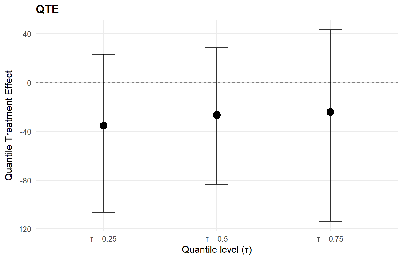
qte_result <- qte(causal_fit, probs = c(0.25, 0.5, 0.75), interval = "credible")
att_result <- att(causal_fit, interval = "credible", nsim_mean = 50)
qtt_result <- qtt(causal_fit, probs = c(0.25, 0.5, 0.75), interval = "credible")
ate_rmean_result <- ate_rmean(causal_fit, cutoff = 10, interval = "credible", nsim_mean = 50)
cate_result <- cate(causal_fit, newdata = X_causal[1:5, ], interval = "credible", nsim_mean = 50)
cqte_result <- cqte(causal_fit, probs = c(0.25, 0.5, 0.75), newdata = X_causal[1:5, ], interval = "credible")
att_rmean_result <- att(causal_fit, type = "rmean", cutoff = 10, interval = "credible", nsim_mean = 50)
cate_rmean_result <- cate(causal_fit, type = "rmean", cutoff = 10, newdata = X_causal[1:5, ], interval = "credible", nsim_mean = 50)

print(ate_result)

ATE (Average Treatment Effect) Prediction points: 1 Conditional (covariates): NO Propensity score used: YES PS scale: logit Posterior mean draws: 50 Credible interval: credible (95%)

ATE estimates (treated - control): id mean lower upper 1 -32.154 -96.251 35.272

Code

summary(ate_result)

ATE Summary

Prediction points: 1 Conditional: NO | PS used: YES Posterior mean draws: 50 Interval: credible (95%)

Model specification: Backend (trt/con): sb / sb Kernel (trt/con): normal / laplace GPD tail (trt/con): NO / NO

ATE statistics: Mean: -32.154 | Median: -32.154 Range: [-32.154, -32.154]

Credible interval width: Mean: 131.523 | Median: 131.523 Range: [131.523, 131.523]

Code

print(ate_rmean_result)

RMCATE (Conditional Restricted Mean Treatment Effect) Prediction points: 32 Conditional (covariates): YES Propensity score used: YES PS scale: logit Posterior mean draws: 50 Credible interval: credible (95%)

RMCATE estimates (treated - control): id mean lower upper 1 -17.695 -65.018 11.262 2 -17.742 -64.951 11.352 3 -12.17 -48.478 13.998 4 -16.61 -62.415 13.603 5 -34.03 -115.333 5.736 6 -15.259 -58.254 14.417 … (26 more rows)

Code

summary(ate_rmean_result)

RMCATE Summary

Prediction points: 32 Conditional: YES | PS used: YES Posterior mean draws: 50 Interval: credible (95%)

Model specification: Backend (trt/con): sb / sb Kernel (trt/con): normal / laplace GPD tail (trt/con): NO / NO

RMCATE statistics: Mean: -26.771 | Median: -20.854 Range: [-71.496, -2.815] SD: 17.563

Credible interval width: Mean: 100.095 | Median: 84.733 Range: [36.907, 217.242]

Code

print(att_rmean_result)

RMATT (Restricted Mean Treatment Effect on the Treated) Prediction points: 1 Conditional (covariates): NO Propensity score used: YES PS scale: logit Posterior mean draws: 50 Credible interval: credible (95%)

RMATT estimates (treated - control): id mean lower upper 1 -21.212 -73.244 10.109

Code

print(cate_rmean_result)

RMCATE (Conditional Restricted Mean Treatment Effect) Prediction points: 5 Conditional (covariates): YES Propensity score used: YES PS scale: logit Posterior mean draws: 50 Credible interval: credible (95%)

RMCATE estimates (treated - control): id mean lower upper 1 -17.693 -64.995 11.211 2 -17.76 -65.033 11.31 3 -12.178 -48.47 13.954 4 -16.624 -62.45 13.593 5 -34.038 -115.466 5.808

Code


plot(ate_result, type = "effect")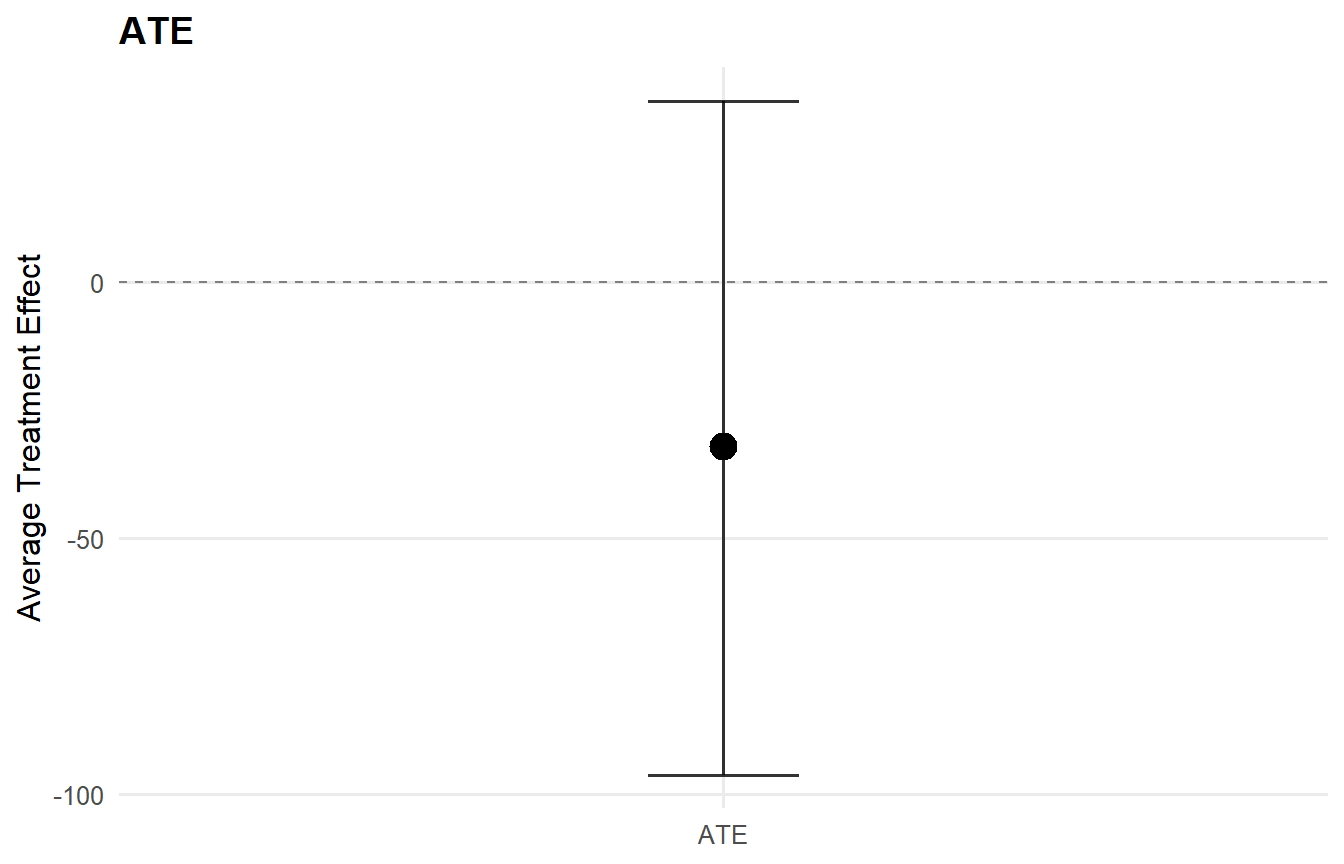

Code

plot(qte_result, type = "effect")

Prereqs

Required packages and data for this page are listed in the setup chunks above.

Outputs

This page renders model fits, diagnostics, and summary artifacts generated by package APIs.

Interpretation

Canonical concept page: Customization And Tuning
Treat this page as an application/example view and use the canonical page for core definitions.

Continue to the linked canonical concept page, then return for implementation-specific details.

Overview

Data

SB Case: Manual Stick-Breaking Model with dNormMix

Note on custom likelihoods

Constants, data, and inits

NIMBLE code

Compile and run (manual)

Sample extraction

Optional: S3 methods via the CausalMixGPD bundle

SB + GPD Case: Manual Pipeline with Codegen

Specification

Build bundle and extract pieces

Compile and run (manual)

Sample extraction

S3 methods for posterior inference

Causal Model: From Bundle to S3 Inference

ATE Summary

RMCATE Summary

Prereqs

Outputs

Interpretation

Next

SB Case: Manual Stick-Breaking Model with `dNormMix`