flowchart TD
  Data[Data: y and optional X] --> Build[Build: bundle()/build_*_bundle()]
  Build --> Fit[Fit: dpmix()/dpmgpd()/dpmix.causal()/dpmgpd.causal()]

  Fit --> Consumers[Consumers: S3 methods]
  Consumers --> Summ[summary()/params()]
  Consumers --> Pred[predict()]
  Consumers --> Plots[plot()]

  Build --> Spec[param_specs: fixed/dist/link/link+dist]
  Spec --> Bulk[Bulk kernel plan]
  Spec --> Tail[GPD tail plan (optional)]

  Bulk --> Model[Outcome model]
  Tail --> Model
  Model --> Fit
Model Umbrella: Custom Models (All-in-One)
Overview
This vignette collects two end-to-end examples with customized priors and links:
- Conditional CRP + Amoroso + GPD with covariates, custom links, and tail settings.
- Causal model (two arms) with SB backends: Normal (treated) and Laplace (control), with covariate-linked locations and custom priors.
Both examples use mtcars and show the main user-level functions plus S3 methods (print, summary, plot, predict, fitted, residuals, params, ate, qte, att, qtt, cate, cqte, ate_rmean).
For causal estimands: cate() / cqte() are conditional and require X; they use newdata when supplied and otherwise training X. ate() / att() / qte() / qtt() are marginal and always use training data (any supplied newdata/y is ignored with a warning). Mean-based R-mean estimands are available through type = "rmean" and ate_rmean().
Note on link priors: both SB and CRP backends currently require normal priors for link-mode regression coefficients. The requested lognormal prior for the scale link is therefore shown below as a non-executed spec block.
How to read this page
This page is the “umbrella” for advanced use:
- It shows where you customize (mostly via
param_specsand the wrapper/bundle interface). - It shows what you get back (fit objects + S3 methods).
- It is intentionally end-to-end so other pages can link here rather than repeating the full picture.
Model decomposition (canonical map)
ImportantDeveloper notes
If you are extending kernels/tails or adding new supported prediction types, keep this decomposition stable: registries define support and defaults; bundle builders normalize specs; runners produce fits; consumers read fits.
Data
Code
data("mtcars", package = "datasets")
df <- mtcars
y <- df$mpg
X <- df[, c("wt", "hp")]
X <- as.data.frame(X)
Model 1: CRP + Amoroso + GPD (Conditional)
Specification
- Backend: CRP
- Kernel: Amoroso
- Covariates:
wt,hp
- Bulk:
loc: identity link, normal prior on coefficientsscale: identity link, normal prior on coefficients (CRP restriction)shape1: fixed at 1shape2: default prior
- Tail:
threshold: exp link, normal prior on coefficientstail_scale: exp link (default prior)
Code
param_specs_amoroso <- list(
  bulk = list(
    loc = list(
      mode = "link",
      link = "identity",
      beta_prior = list(dist = "normal", args = list(mean = 0, sd = 2))
    ),
    scale = list(
      mode = "link",
      link = "identity",
      beta_prior = list(dist = "normal", args = list(mean = 0, sd = 2))
    ),
    shape1 = list(mode = "fixed", value = 1)
  ),
  gpd = list(
    threshold = list(
      mode = "link",
      link = "exp",
      beta_prior = list(dist = "normal", args = list(mean = 0, sd = 0.2))
    ),
    tail_scale = list(
      mode = "link",
      link = "exp"
    )
  )
)
Code
# Requested variant (not runnable): link-mode beta priors must be normal
param_specs_amoroso_requested <- list(
  bulk = list(
    loc = list(
      mode = "link",
      link = "identity",
      beta_prior = list(dist = "normal", args = list(mean = 0, sd = 2))
    ),
    scale = list(
      mode = "link",
      link = "identity",
      beta_prior = list(dist = "lognormal", args = list(meanlog = 0, sdlog = 1))
    ),
    shape1 = list(mode = "fixed", value = 1)
  ),
  gpd = list(
    threshold = list(
      mode = "link",
      link = "exp",
      beta_prior = list(dist = "normal", args = list(mean = 0, sd = 0.2))
    ),
    tail_scale = list(
      mode = "link",
      link = "exp"
    )
  )
)
Build + Run (CRP note)
NIMBLE’s CRP sampler cannot cluster deterministic nodes created by link-mode parameters. As a result, CRP + covariate links are not runnable with the current backend. We still record the requested CRP specification below (for reference), and then run an SB-equivalent model that supports the same customization and lets this vignette compile end-to-end.
Code
# Requested CRP specification (not runnable due to CRP link-mode restriction)
bundle_amoroso_crp <- bundle(
  y = y,
  X = X,
  backend = "crp",
  kernel = "amoroso",
  GPD = TRUE,
  components = 5,
  param_specs = param_specs_amoroso,
  mcmc = mcmc
)
Code
# Runnable SB equivalent (supports link-mode parameters)
bundle_amoroso <- bundle(
  y = y,
  X = X,
  backend = "sb",
  kernel = "amoroso",
  GPD = TRUE,
  components = 5,
  param_specs = param_specs_amoroso,
  mcmc = mcmc
)

fit_amoroso <- dpmgpd(bundle_amoroso, mcmc = list(show_progress = FALSE))
User-Level Functions
Code
print(bundle_amoroso)CausalMixGPD bundle Field Value Backend Stick-Breaking Process Kernel Amoroso Distribution Components 5 N 32 X YES (P=2) GPD TRUE Epsilon 0.025
contains : code, constants, data, dimensions, inits, monitors
Code
summary(bundle_amoroso)CausalMixGPD bundle summary Field Value Backend Stick-Breaking Process Kernel Amoroso Distribution Components 5 N 32 X YES (P=2) GPD TRUE Epsilon 0.025
Parameter specification block parameter mode level meta backend info model meta kernel info model meta components info model meta N info model meta P info model concentration alpha dist scalar bulk loc link regression bulk scale link regression bulk shape1 fixed component (1:5) bulk shape2 dist component (1:5) gpd threshold link observation (1:N) gpd tail_scale link observation (1:N) gpd tail_shape dist scalar prior link sb
amoroso
5
32
2
gamma(shape=1, rate=1)
beta_loc ~ normal(mean=0, sd=2) identity beta_scale ~ normal(mean=0, sd=2) identity 1
gamma(shape=2, rate=1)
beta_threshold ~ normal(mean=0, sd=0.2) exp beta_tail_scale ~ normal(mean=0, sd=0.5) exp normal(mean=0, sd=0.2)
notes
                               stochastic concentration
                     beta_loc is 5 x 2 (components x P)
                   beta_scale is 5 x 2 (components x P)

                                  iid across components
                           beta_threshold is length P=2
beta_tail_scale is length P=2; tail_scale[i] deterministic
Monitors n = 10 alpha, w[1:5], beta_loc[1:5,1:2], beta_scale[1:5,1:2], shape1[1:5], shape2[1:5], threshold[1:32], beta_threshold[1:2], beta_tail_scale[1:2], tail_shape
Code
print(fit_amoroso)MixGPD fit | backend: Stick-Breaking Process | kernel: Amoroso Distribution | GPD tail: TRUE n = 32 | components = 5 | epsilon = 0.025 MCMC: niter=600, nburnin=150, thin=2, nchains=1 Fit Use summary() for posterior summaries; plot() for diagnostics; predict() for predictions.
Code
summary(fit_amoroso)MixGPD summary | backend: Stick-Breaking Process | kernel: Amoroso Distribution | GPD tail: TRUE | epsilon: 0.025 n = 32 | components = 5 Summary Initial components: 5 | Components after truncation: 2
Summary table parameter mean sd q0.025 q0.500 q0.975 ess weights[1] 0.538 0.153 0.317 0.509 0.829 12.119 weights[2] 0.257 0.077 0.104 0.261 0.395 32.471 alpha 1.539 1.228 0.223 1.233 5.246 10.513 beta_loc[1, 1] 0 0 0 0 0 0 beta_loc[2, 1] 0 0 0 0 0 0 beta_loc[3, 1] 0 0 0 0 0 0 beta_loc[4, 1] 0 0 0 0 0 0 beta_loc[5, 1] 0 0 0 0 0 0 beta_loc[1, 2] 0 0 0 0 0 0 beta_loc[2, 2] 0 0 0 0 0 0 beta_loc[3, 2] 0 0 0 0 0 0 beta_loc[4, 2] 0 0 0 0 0 0 beta_loc[5, 2] 0 0 0 0 0 0 beta_scale[1, 1] -0.135 2.084 -4.366 -0.029 3.689 225 beta_scale[2, 1] -0.004 2.002 -4.287 0.068 4.185 180.011 beta_scale[3, 1] -0.027 1.989 -3.825 0.019 3.567 225 beta_scale[4, 1] -0.079 2.196 -4.33 0.092 3.824 305.837 beta_scale[5, 1] 0.061 1.987 -3.605 -0.031 4.122 225 beta_scale[1, 2] 1.667 1.331 0.027 1.485 4.418 163.395 beta_scale[2, 2] 1.419 1.399 -1.418 1.236 4.328 161.724 beta_scale[3, 2] 1.035 1.694 -2.944 0.984 4.283 148.954 beta_scale[4, 2] 0.578 1.868 -3.302 0.735 4.074 125.824 beta_scale[5, 2] 1.198 1.836 -2.859 1.221 5.031 94.117 beta_tail_scale[1] 0.93 0.192 0.621 0.913 1.333 42.741 beta_tail_scale[2] -0.001 0.004 -0.009 -0.001 0.006 26.472 beta_threshold[1] 0 0 0 0 0 0 beta_threshold[2] 0 0 0 0 0 0 tail_shape 0.301 0.111 0.088 0.289 0.525 157.664 shape1[1] 1 0 1 1 1 0 shape1[2] 1 0 1 1 1 0 shape2[1] 2.563 1.548 0.578 2.217 6.318 64.05 shape2[2] 2.275 1.398 0.397 1.886 5.662 45.533
S3 Methods (Fit)
Code
plot(fit_amoroso, family = "traceplot")
##
## === traceplot ===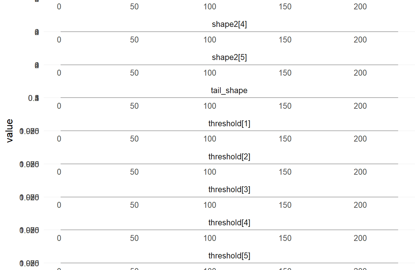
Code
pred_mean <- predict(
  fit_amoroso,
  x = X,
  type = "mean",
  level = 0.90,
  interval = "credible",
  workers = max_workers,
  ndraws_pred = 200,
  chunk_size = 10000
)
pred_q90 <- predict(fit_amoroso, newdata =X, type = "quantile", p = 0.90, level = 0.90, interval = "credible", workers = max_workers)
head(pred_mean$fit)
##   id estimate     lower    upper
## 1  1 18.36918 10.848036 34.57267
## 2  2 22.57066 13.166294 39.36972
## 3  3 14.20863  8.851946 23.45784
## 4  4 30.60308 17.557581 48.27957
## 5  5 35.80440 19.435758 68.89430
## 6  6 37.22761 19.725989 66.63192
head(pred_q90$fit)
##   id index estimate    lower     upper
## 1  1   0.9 35.73854 25.04434  47.18495
## 2  2   0.9 45.28021 29.64321  61.68626
## 3  3   0.9 27.58261 19.74898  35.58991
## 4  4   0.9 62.42953 36.58253  91.81649
## 5  5   0.9 72.50266 45.36133 107.34721
## 6  6   0.9 79.60537 42.08101 131.73323
Code
ess_amoroso <- ess_summary(fit_amoroso)
print(ess_amoroso)
## ESS summary (ESS/sec)
##     arm              param  chain     ess seconds ess_per_sec
##  single              alpha chain1  10.513    0.94      11.184
##  single         tail_shape chain1 157.664    0.94     167.728
##  single beta_tail_scale[1] chain1  42.741    0.94      45.469
##  single              alpha pooled  10.513    0.94      11.184
##  single         tail_shape pooled 157.664    0.94     167.728
##  single beta_tail_scale[1] pooled  42.741    0.94      45.469
Code
fvals <- fitted(fit_amoroso, type = "mean", level = 0.90)
head(fvals)
##        fit     lower    upper   residuals
## 1 17.53502 11.055603 29.46088   3.4649815
## 2 20.78361 13.157036 37.89295   0.2163936
## 3 14.54645  9.234695 26.33764   8.2535461
## 4 31.01728 17.198270 49.40405  -9.6172813
## 5 34.50765 20.424316 58.08441 -15.8076534
## 6 37.48254 19.731315 63.00764 -19.3825399
summary(fvals$residuals)
##    Min. 1st Qu.  Median    Mean 3rd Qu.    Max.
## -191.31  -23.44  -11.98  -22.06    5.96   35.09
Code
raw_resid <- residuals(fit_amoroso, type = "raw")
head(raw_resid)
## [1]   3.4649815   0.2163936   8.2535461  -9.6172813 -15.8076534 -19.3825399
Code
p <- params(fit_amoroso)
names(p)
## [1] "alpha"           "w"               "beta_loc"        "beta_scale"
## [5] "shape1"          "shape2"          "beta_threshold"  "beta_tail_scale"
## [9] "tail_shape"
Model 2: Causal (SB Normal vs SB Laplace)
Specification
- Backend: SB (both arms)
- Treated arm (A=1): Normal kernel
- Location: identity link, Gaussian prior
- SD: Inverse-Gamma prior
- Location: identity link, Gaussian prior
- Control arm (A=0): Laplace kernel
- Location: identity link, Gaussian prior
- Scale: Gamma prior
- Location: identity link, Gaussian prior
For the causal building blocks behind these two-arm models (potential outcomes, propensity-score augmentation) and the interpretation of the reported estimands, see: - Theory: Causal objects (potential outcomes + estimands) - Theory: Restricted means, extreme quantiles, and interpretation
Code
X_causal <- df[, c("wt", "hp", "qsec", "cyl")]
X_causal <- as.data.frame(X_causal)
T_ind <- df$am

param_specs_causal <- list(
  trt = list(
    bulk = list(
      mean = list(
        mode = "link",
        link = "identity",
        beta_prior = list(dist = "normal", args = list(mean = 0, sd = 2))
      ),
      sd = list(
        mode = "dist",
        dist = "invgamma",
        args = list(shape = 2, scale = 1)
      )
    )
  ),
  con = list(
    bulk = list(
      location = list(
        mode = "link",
        link = "identity",
        beta_prior = list(dist = "normal", args = list(mean = 0, sd = 2))
      ),
      scale = list(
        mode = "dist",
        dist = "gamma",
        args = list(shape = 2, rate = 1)
      )
    )
  )
)
Build + Run
Code
causal_bundle <- build_causal_bundle(
  y = y,
  X = X_causal,
  A = T_ind,
  backend = "sb",
  kernel = c("normal", "laplace"),
  GPD = FALSE,
  components = 5,
  param_specs = param_specs_causal,
  PS = "logit",
  mcmc_outcome = mcmc,
  mcmc_ps = mcmc
)

causal_fit <- dpmix.causal(causal_bundle, mcmc = causal_run_mcmc)
User-Level Functions
Code
print(causal_bundle)CausalMixGPD causal bundle PS model: Bayesian logit (A | X) Field Treated Control Backend Stick-Breaking Process Stick-Breaking Process Kernel normal laplace Components 5 5 GPD tail FALSE FALSE Epsilon 0.025 0.025
Outcome PS included: TRUE n (control) = 19 | n (treated) = 13
Code
summary(causal_bundle)CausalMixGPD causal bundle summary CausalMixGPD causal bundle PS model: Bayesian logit (A | X) Field Treated Control Backend Stick-Breaking Process Stick-Breaking Process Kernel normal laplace Components 5 5 GPD tail FALSE FALSE Epsilon 0.025 0.025
Outcome PS included: TRUE n (control) = 19 | n (treated) = 13
Code
print(causal_fit)CausalMixGPD causal fit PS model: Bayesian logit (A | X) Outcome (treated): backend = sb | kernel = normal Outcome (control): backend = sb | kernel = laplace GPD tail (treated/control): FALSE / FALSE
Code
summary(causal_fit)– PS fit – CausalMixGPD PS fit model: logit
– Outcome fits – [control] MixGPD fit | backend: Stick-Breaking Process | kernel: Laplace Distribution | GPD tail: FALSE n = 19 | components = 5 | epsilon = 0.025 MCMC: niter=600, nburnin=150, thin=2, nchains=1 Fit Use summary() for posterior summaries; plot() for diagnostics; predict() for predictions.
[treated] MixGPD fit | backend: Stick-Breaking Process | kernel: Normal Distribution | GPD tail: FALSE n = 13 | components = 5 | epsilon = 0.025 MCMC: niter=600, nburnin=150, thin=2, nchains=1 Fit Use summary() for posterior summaries; plot() for diagnostics; predict() for predictions.
S3 Methods (Causal)
Code
plot(causal_fit, family = "traceplot")
##
## === treated ===
##
## === traceplot ===
##
## === control ===
##
## === traceplot ===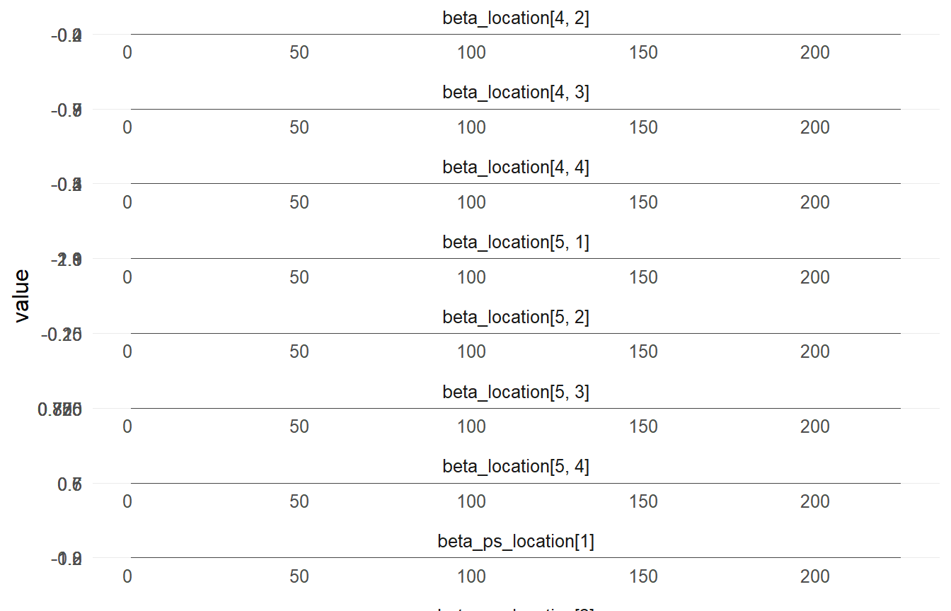
Code
pred_causal_mean <- predict(causal_fit, newdata =X_causal, type = "mean", interval = "credible", workers = max_workers)
head(pred_causal_mean)
##   id  estimate     lower    upper        ps
## 1  1  68.62577  85.15852 53.15772 0.5098190
## 2  2  68.87877  85.35540 53.36696 0.3673327
## 3  3  58.41981  72.25273 46.06000 0.6671039
## 4  4  70.47160  86.29427 54.47266 0.2529819
## 5  5 101.76433 126.62140 79.08810 0.2699014
## 6  6  68.36559  82.98814 53.21215 0.1616853
Code
ess_causal <- ess_summary(causal_fit)
print(ess_causal)
## ESS summary (ESS/sec)
##      arm               param  chain    ess seconds ess_per_sec
##  control               alpha chain1 23.939    0.06     398.986
##  control            scale[1] chain1 57.736    0.06     962.264
##  control beta_ps_location[1] chain1  1.512    0.06      25.203
##  control               alpha pooled 23.939    0.06     398.986
##  control            scale[1] pooled 57.736    0.06     962.264
##  control beta_ps_location[1] pooled  1.512    0.06      25.203
##  treated               alpha chain1  45.78    0.03    1525.993
##  treated     beta_ps_mean[1] chain1  2.606    0.03      86.878
##  treated               alpha pooled  45.78    0.03    1525.993
##  treated     beta_ps_mean[1] pooled  2.606    0.03      86.878
Code
ate_result <- ate(causal_fit, interval = "credible", nsim_mean = 50)
att_result <- att(causal_fit, interval = "credible", nsim_mean = 50)
ate_rmean_result <- ate_rmean(causal_fit, cutoff = 10, interval = "credible", nsim_mean = 50)
att_rmean_result <- att(causal_fit, type = "rmean", cutoff = 10, interval = "credible", nsim_mean = 50)
cate_rmean_result <- cate(causal_fit, type = "rmean", cutoff = 10, newdata = X_causal[1:5, ], interval = "credible", nsim_mean = 50)
print(ate_result)
ATE (Average Treatment Effect) Prediction points: 1 Conditional (covariates): NO Propensity score used: YES PS scale: logit Posterior mean draws: 50 Credible interval: credible (95%)
ATE estimates (treated - control): id mean lower upper 1 86.066 13.386 157.707
Code
summary(ate_result)ATE Summary
Prediction points: 1 Conditional: NO | PS used: YES Posterior mean draws: 50 Interval: credible (95%)
Model specification: Backend (trt/con): sb / sb Kernel (trt/con): normal / laplace GPD tail (trt/con): NO / NO
ATE statistics: Mean: 86.066 | Median: 86.066 Range: [86.066, 86.066]
Credible interval width: Mean: 144.321 | Median: 144.321 Range: [144.321, 144.321]
Code
print(ate_rmean_result)RMCATE (Conditional Restricted Mean Treatment Effect) Prediction points: 32 Conditional (covariates): YES Propensity score used: YES PS scale: logit Posterior mean draws: 50 Credible interval: credible (95%)
RMCATE estimates (treated - control): id mean lower upper 1 45.808 -4.652 94.66 2 46.409 -4.933 95.068 3 38.231 -3.464 77.773 4 46.29 -4.299 93.94 5 66.163 -16.159 144.307 6 45.631 -1.534 91.492 … (26 more rows)
Code
summary(ate_rmean_result)RMCATE Summary
Prediction points: 32 Conditional: YES | PS used: YES Posterior mean draws: 50 Interval: credible (95%)
Model specification: Backend (trt/con): sb / sb Kernel (trt/con): normal / laplace GPD tail (trt/con): NO / NO
RMCATE statistics: Mean: 56.224 | Median: 49.96 Range: [26.903, 107.303] SD: 20.473
Credible interval width: Mean: 133.518 | Median: 112.24 Range: [44.786, 308.927]
Code
print(att_rmean_result)RMATT (Restricted Mean Treatment Effect on the Treated) Prediction points: 1 Conditional (covariates): NO Propensity score used: YES PS scale: logit Posterior mean draws: 50 Credible interval: credible (95%)
RMATT estimates (treated - control): id mean lower upper 1 48.603 -8.89 103.589
Code
print(cate_rmean_result)RMCATE (Conditional Restricted Mean Treatment Effect) Prediction points: 5 Conditional (covariates): YES Propensity score used: YES PS scale: logit Posterior mean draws: 50 Credible interval: credible (95%)
RMCATE estimates (treated - control): id mean lower upper 1 45.941 -5.517 95.245 2 46.117 -6.108 95.36 3 38.476 -2.935 78.753 4 46.962 -3.633 95.922 5 65.817 -16.61 144.573
Code
qte_result <- qte(causal_fit, probs = c(0.25, 0.5, 0.75), interval = "credible")
qtt_result <- qtt(causal_fit, probs = c(0.25, 0.5, 0.75), interval = "credible")
cqte_result <- cqte(causal_fit, probs = c(0.25, 0.5, 0.75), newdata = X_causal[1:5, ], interval = "credible")
cate_result <- cate(causal_fit, newdata = X_causal[1:5, ], interval = "credible", nsim_mean = 50)
plot(ate_result, type = "effect")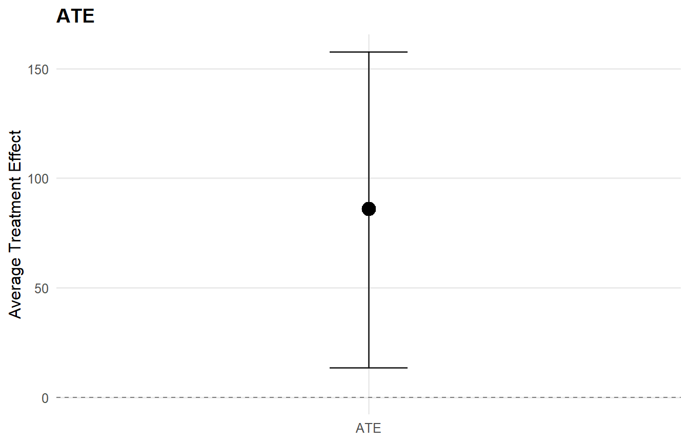
Code
plot(qte_result, type = "effect")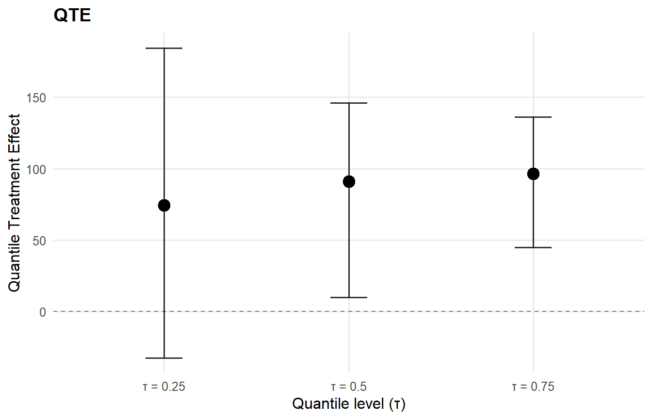
Prereqs
- Required packages and data for this page are listed in the setup chunks above.
Outputs
- This page renders model fits, diagnostics, and summary artifacts generated by package APIs.
Interpretation
- Canonical concept page: Model Umbrella
- Treat this page as an application/example view and use the canonical page for core definitions.
Next
- Continue to the linked canonical concept page, then return for implementation-specific details.