Inverse Gaussian (base kernel)

Inverse Gaussian base kernel (single component)

This section documents the same inverse Gaussian density as above, but for a single component rather than a mixture: [ f(y,) = ()^{1/2} !(-), y>0. ]

Parameter mapping (math () code): () mean, () shape.

Inverse Gaussian base with GPD tail

The dInvGaussGpd, pInvGaussGpd, qInvGaussGpd, and rInvGaussGpd functions splice the base inverse Gaussian below (u) with a GPD tail above (u).

Tail mapping (math () code): (u) threshold, () tail_scale, () tail_shape.

Without GPD

Code

grid <- seq(0.1, 6, length.out = 400)
ig_base_sets <- list(
  list(label = "Base A", mean = 1.2, shape = 3.0),
  list(label = "Base B", mean = 1.5, shape = 4.0),
  list(label = "Base C", mean = 1.0, shape = 2.5)
)

example <- ig_base_sets[[1]]

Code

dInvGauss(1, mean = example$mean, shape = example$shape)

[1] 0.6627887

Code

dInvGauss(1, mean = example$mean, shape = example$shape, log = TRUE)

[1] -0.4112991

Code

pInvGauss(1, mean = example$mean, shape = example$shape)

[1] 0.4974402

Code

pInvGauss(1, mean = example$mean, shape = example$shape, lower.tail = FALSE)

[1] 0.5025598

Code

pInvGauss(1, mean = example$mean, shape = example$shape, log.p = TRUE)

[1] -0.6982799

Code

q_vec(qInvGauss, c(0.25, 0.5, 0.75), mean = example$mean,
      shape = example$shape)

[1] 0.6732028 1.0038699 1.5093817

Code

q_vec(qInvGauss, c(0.25, 0.5, 0.75), mean = example$mean,
      shape = example$shape, lower.tail = FALSE)

[1] 1.5093817 1.0038699 0.6732028

Code

q_vec(qInvGauss, c(log(0.25), log(0.5), log(0.75)), mean = example$mean,
      shape = example$shape, log.p = TRUE)

[1] 0.6732028 1.0038699 1.5093817

Code

draw_many(rInvGauss, list(mean = example$mean, shape = example$shape))

[1] 0.8095021 2.7192599 0.4547103 0.4691927 1.6313223

Code

df_ig_base <- do.call(rbind, lapply(ig_base_sets, function(ps) {
  data.frame(x = grid, density = density_curve(grid, dInvGauss, list(mean = ps$mean, shape = ps$shape)), label = ps$label)
}))

ggplot(df_ig_base, aes(x = x, y = density, color = label)) +
  geom_line(linewidth = 1) +
  labs(title = "Inverse Gaussian base kernels", x = "x", y = "density") +
  theme_minimal() + theme(legend.position = "top")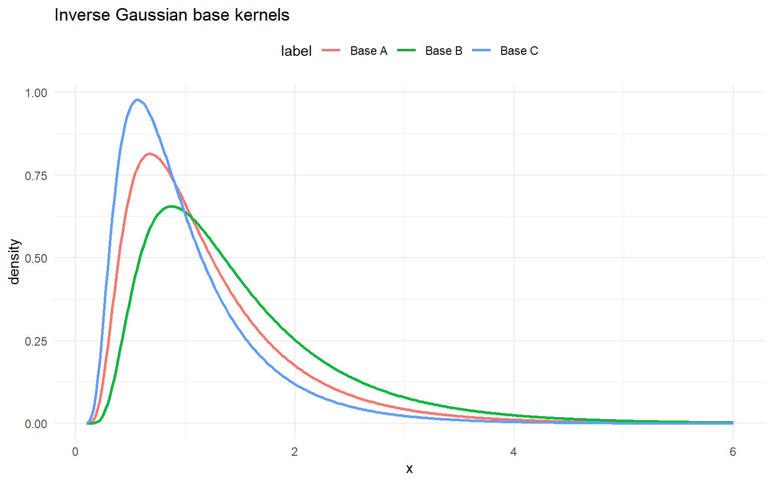

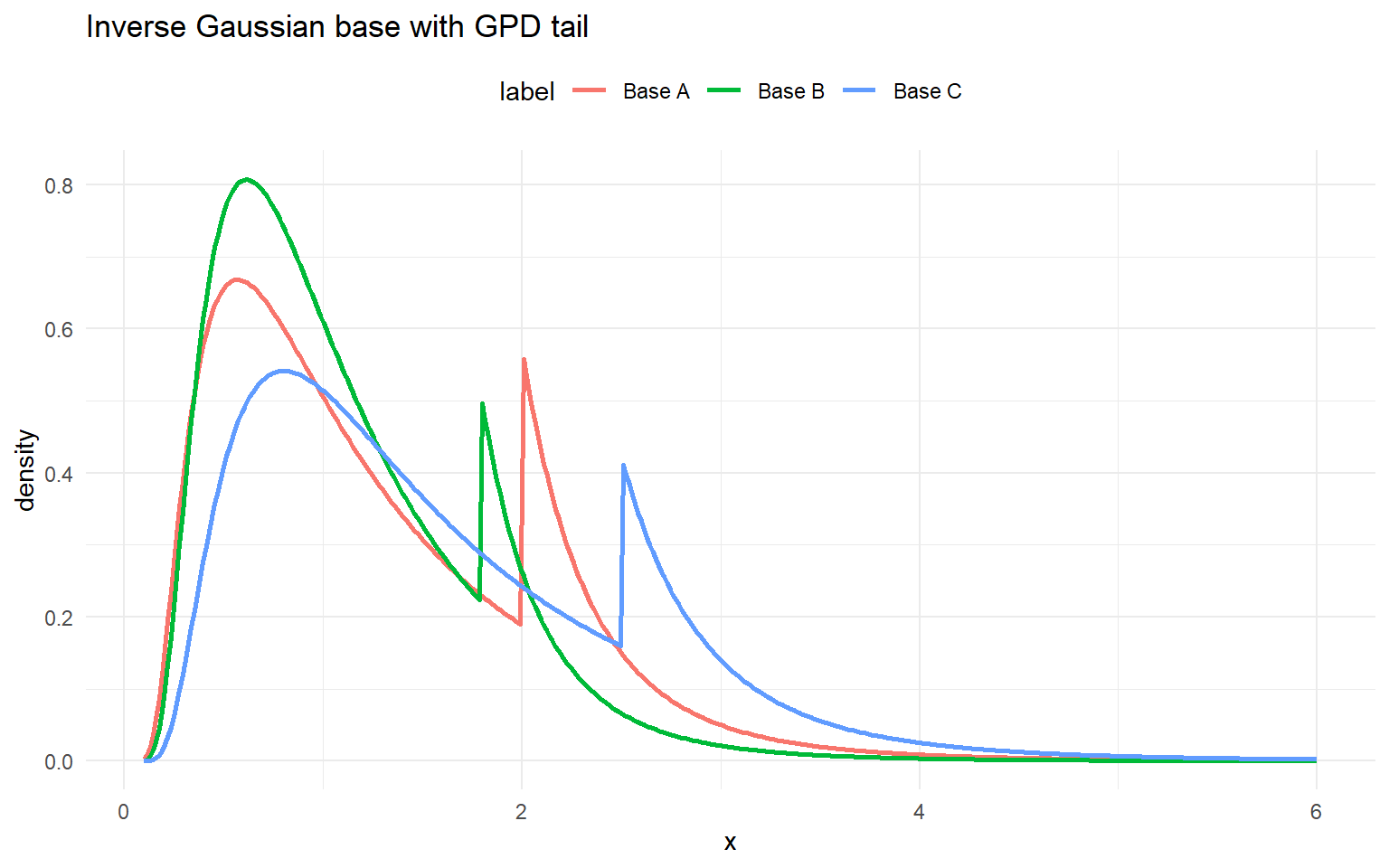
With GPD tail

Code

ig_base_gpd_sets <- list(
  list(label = "Base A", mean = 1.5, shape = 2, threshold = 2.0, tail_scale = 0.4, tail_shape = 0.2),
  list(label = "Base B", mean = 1.2, shape = 2.5, threshold = 1.8, tail_scale = 0.35, tail_shape = 0.18),
  list(label = "Base C", mean = 1.8, shape = 3, threshold = 2.5, tail_scale = 0.5, tail_shape = 0.22)
)
example <- ig_base_gpd_sets[[1]]

Code

dInvGaussGpd(2, mean = example$mean, shape = example$shape,
             threshold = example$threshold, tail_scale = example$tail_scale,
             tail_shape = example$tail_shape)

[1] 0.5704499

Code

dInvGaussGpd(2, mean = example$mean, shape = example$shape,
             threshold = example$threshold, tail_scale = example$tail_scale,
             tail_shape = example$tail_shape, log = TRUE)

[1] -0.56133

Code

pInvGaussGpd(2, mean = example$mean, shape = example$shape,
             threshold = example$threshold, tail_scale = example$tail_scale,
             tail_shape = example$tail_shape)

[1] 0.77182

Code

pInvGaussGpd(2, mean = example$mean, shape = example$shape,
             threshold = example$threshold, tail_scale = example$tail_scale,
             tail_shape = example$tail_shape, lower.tail = FALSE)

[1] 0.22818

Code

pInvGaussGpd(2, mean = example$mean, shape = example$shape,
             threshold = example$threshold, tail_scale = example$tail_scale,
             tail_shape = example$tail_shape, log.p = TRUE)

[1] -0.2590039

Code

q_vec(qInvGaussGpd, c(0.25, 0.5, 0.75), mean = example$mean,
      shape = example$shape, threshold = example$threshold,
      tail_scale = example$tail_scale, tail_shape = example$tail_shape)

[1] 0.6561675 1.1013488 1.8902777

Code

q_vec(qInvGaussGpd, c(0.25, 0.5, 0.75), mean = example$mean,
      shape = example$shape, threshold = example$threshold,
      tail_scale = example$tail_scale, tail_shape = example$tail_shape,
      lower.tail = FALSE)

[1] 1.8902777 1.1013488 0.6561675

Code

q_vec(qInvGaussGpd, c(log(0.25), log(0.5), log(0.75)), mean = example$mean,
      shape = example$shape, threshold = example$threshold,
      tail_scale = example$tail_scale, tail_shape = example$tail_shape,
      log.p = TRUE)

[1] 0.6561675 1.1013488 1.8902777

Code

draw_many(rInvGaussGpd, example)

[1] 0.9156239 3.4518691 1.0719015 8.2451188 1.4427542

Code

df_ig_base_gpd <- do.call(rbind, lapply(ig_base_gpd_sets, function(ps) {
  data.frame(x = grid, density = density_curve(grid, dInvGaussGpd, list(mean = ps$mean, shape = ps$shape, threshold = ps$threshold, tail_scale = ps$tail_scale, tail_shape = ps$tail_shape)), label = ps$label)
}))

ggplot(df_ig_base_gpd, aes(x = x, y = density, color = label)) +
  geom_line(linewidth = 1) +
  labs(title = "Inverse Gaussian base with GPD tail", x = "x", y = "density") +
  theme_minimal() + theme(legend.position = "top")

Prereqs

Required packages and data for this page are listed in the setup chunks above.

Outputs

This page renders model fits, diagnostics, and summary artifacts generated by package APIs.

Interpretation

Canonical concept page: Introduction With Gpd Kernel
Treat this page as an application/example view and use the canonical page for core definitions.

Continue to the linked canonical concept page, then return for implementation-specific details.