Inverse Gaussian (mixture kernel)

Inverse Gaussian mixture kernel (finite components)

An inverse Gaussian component with mean (>0) and shape (>0) has density [ f(y,) = ()^{1/2} !(-), y>0. ]

A finite inverse Gaussian mixture is [ f(y)=_{j=1}^J w_j,(y_j,_j),y>0. ]

Parameter mapping (math () code): (_j) mean[j], (_j) shape[j], (w_j) w[j].

Inverse Gaussian mixture with GPD tail

The spliced variant attaches a GPD tail above (u).

Tail mapping (math () code): (u) threshold, () tail_scale, () tail_shape.

Without GPD

Code

grid <- seq(0.1, 6, length.out = 400)
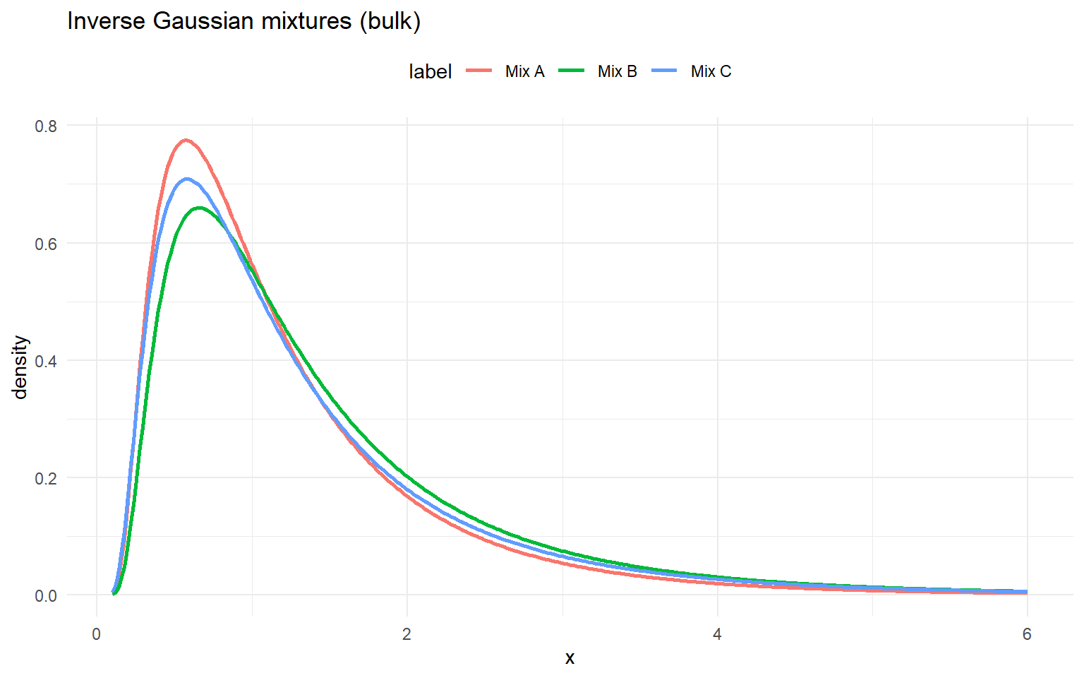
ig_sets <- list(
  list(label = "Mix A", w = c(0.6, 0.3, 0.1), mean = c(1.0, 1.5, 2.0), shape = c(2.0, 3.0, 4.0)),
  list(label = "Mix B", w = c(0.5, 0.3, 0.2), mean = c(1.1, 1.6, 2.2), shape = c(2.2, 3.2, 4.2)),
  list(label = "Mix C", w = c(0.4, 0.35, 0.25), mean = c(0.9, 1.4, 2.1), shape = c(1.8, 2.8, 3.8))
)

example <- ig_sets[[1]]

Code

dInvGaussMix(1, w = example$w, mean = example$mean, shape = example$shape)

[1] 0.5623806

Code

dInvGaussMix(1.5, w = example$w, mean = example$mean, shape = example$shape, log = TRUE)

[1] -1.175151

Code

pInvGaussMix(1.5, w = example$w, mean = example$mean, shape = example$shape)

[1] 0.7287565

Code

pInvGaussMix(1.5, w = example$w, mean = example$mean, shape = example$shape, lower.tail = FALSE)

[1] 0.2712435

Code

pInvGaussMix(1.5, w = example$w, mean = example$mean, shape = example$shape, log.p = TRUE)

[1] -0.3164157

Code

q_vec(qInvGaussMix, c(0.25, 0.5, 0.75), w = example$w, mean = example$mean,
      shape = example$shape)

[1] 0.6082680 0.9714913 1.5718861

Code

q_vec(qInvGaussMix, c(0.25, 0.5, 0.75), w = example$w, mean = example$mean,
      shape = example$shape, lower.tail = FALSE)

[1] 1.5718861 0.9714913 0.6082680

Code

q_vec(qInvGaussMix, c(log(0.25), log(0.5), log(0.75)), w = example$w,
      mean = example$mean, shape = example$shape, log.p = TRUE)

[1] 0.6082680 0.9714913 1.5718861

Code

draw_many(rInvGaussMix, list(w = example$w, mean = example$mean, shape = example$shape))

[1] 1.2588182 0.4181708 0.5295295 1.2182819 0.3206921

Code

df_ig <- do.call(rbind, lapply(ig_sets, function(ps) {
  data.frame(x = grid, density = density_curve(grid, dInvGaussMix, list(w = ps$w, mean = ps$mean, shape = ps$shape)), label = ps$label)
}))

ggplot(df_ig, aes(x = x, y = density, color = label)) +
  geom_line(linewidth = 1) +
  labs(title = "Inverse Gaussian mixtures (bulk)", x = "x", y = "density") +
  theme_minimal() + theme(legend.position = "top")

With GPD tail

Code

ig_gpd_sets <- list(
  list(label = "Mix A", w = c(0.6, 0.4), mean = c(1, 2.5), shape = c(2, 3), threshold = 2.5, tail_scale = 0.5, tail_shape = 0.25),
  list(label = "Mix B", w = c(0.5, 0.5), mean = c(1.5, 2), shape = c(2.5, 2.5), threshold = 2.0, tail_scale = 0.4, tail_shape = 0.2),
  list(label = "Mix C", w = c(0.7, 0.3), mean = c(1.2, 3), shape = c(3, 2), threshold = 3.0, tail_scale = 0.6, tail_shape = 0.18)
)

example <- ig_gpd_sets[[1]]

Code

dInvGaussMixGpd(2.5, w = example$w, mean = example$mean, shape = example$shape, threshold = example$threshold, tail_scale = example$tail_scale, tail_shape = example$tail_shape)

[1] 0.3251727

Code

pInvGaussMixGpd(2.5, w = example$w, mean = example$mean, shape = example$shape, threshold = example$threshold, tail_scale = example$tail_scale, tail_shape = example$tail_shape)

[1] 0.8374137

Code

q_vec(qInvGaussMixGpd, c(0.5, 0.9), w = example$w, mean = example$mean, shape = example$shape, threshold = example$threshold, tail_scale = example$tail_scale, tail_shape = example$tail_shape)

[1] 1.061874 2.758401

Code

draw_many(rInvGaussMixGpd, example)

[1] 2.6228440 0.6467303 3.6319603 1.9262774 3.0668854

Code

df_ig_gpd <- do.call(rbind, lapply(ig_gpd_sets, function(ps) {
  data.frame(x = grid, density = density_curve(grid, dInvGaussMixGpd, list(w = ps$w, mean = ps$mean, shape = ps$shape, threshold = ps$threshold, tail_scale = ps$tail_scale, tail_shape = ps$tail_shape)), label = ps$label)
}))

ggplot(df_ig_gpd, aes(x = x, y = density, color = label)) +
  geom_line(linewidth = 1) +
  labs(title = "Inverse Gaussian mixtures with GPD tail", x = "x", y = "density") +
  theme_minimal() + theme(legend.position = "top")

Prereqs

Required packages and data for this page are listed in the setup chunks above.

Outputs

This page renders model fits, diagnostics, and summary artifacts generated by package APIs.

Interpretation

Canonical concept page: Introduction With Gpd Kernel
Treat this page as an application/example view and use the canonical page for core definitions.

Continue to the linked canonical concept page, then return for implementation-specific details.

Inverse Gaussian (mixture kernel)

Inverse Gaussian mixture kernel (finite components)

Inverse Gaussian mixture with GPD tail

Without GPD

With GPD tail

Prereqs

Outputs

Interpretation

Next