ex01. Unconditional DPM (CRP Backend)

Website workflow note. This page reflects the current exported API and recommended wrapper-first usage. Last updated: 2026-02-19.

For the full package narrative, see the main package vignettes (basic, unconditional, conditional, and causal).

Unconditional DPmix: Chinese Restaurant Process (CRP)

What you’ll learn

Fit a bulk-only one-arm model with dpmix() using the CRP backend.
Use the package’s S3 surface (summary(), plot(), predict()) to diagnose and extract posterior predictive summaries.

When to use this template

You have a single outcome (y) and want a flexible density model without covariates (X).
You do not need tail splicing (GPD = FALSE).
You want adaptive clustering behavior via CRP (within a finite components cap).

Goal (in one sentence)

Estimate the density of a univariate outcome (y) using a Dirichlet-process mixture with a Chinese Restaurant Process backend.

Model: \(y_i | G \sim \int K(y_i; \theta) dG(\theta)\) where \(G \sim \text{DP}(\alpha, G_0)\)

Backend: CRP with truncation at max components

Data Setup

Code

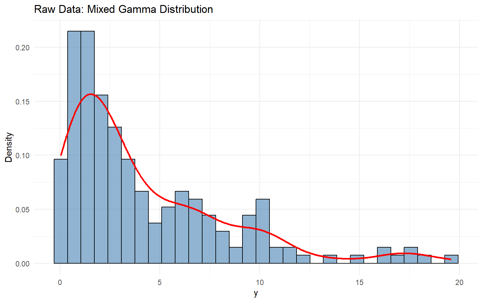
# Load pre-generated dataset: 200 observations from mixture of 3 gamma components
data("nc_pos200_k3")
y_mixed <- nc_pos200_k3$y

paste("Sample size:", length(y_mixed))

[1] "Sample size: 200"

Code

paste("Mean:", mean(y_mixed))

[1] "Mean: 4.21476750434594"

Code

paste("SD:", sd(y_mixed))

[1] "SD: 4.10835046697183"

Code

paste("Range:", paste(range(y_mixed), collapse = " to "))

[1] "Range: 0.0403111680208858 to 19.6013451514889"

Code

# Visualization
df_data <- data.frame(y = y_mixed)
p_raw <- ggplot(df_data, aes(x = y)) +
  geom_histogram(aes(y = after_stat(density)), bins = 30, alpha = 0.6, fill = "steelblue",color = "black") +
  geom_density(color = "red", linewidth = 1) +
  labs(title = "Raw Data: Mixed Gamma Distribution", x = "y", y = "Density") +
  theme_minimal()

print(p_raw)

Model Specification & Bundle

This page keeps the direct bundle() workflow because it is still useful for showing how the unconditional CRP specification is assembled before fitting.

Code

bundle_crp <- bundle(
  y = y_mixed,
  kernel = "laplace",
  backend = "crp",
  GPD = FALSE,
  components = 3,
  alpha_random = TRUE,
  mcmc = mcmc
)

Summary of MCMC Bundle

Code

summary(bundle_crp)

CausalMixGPD bundle summary
      Field                      Value
    Backend Chinese Restaurant Process
     Kernel       Laplace Distribution
 Components                          3
          N                        200
          X                         NO
        GPD                      FALSE
    Epsilon                      0.025

Parameter specification
         block  parameter mode           level                  prior link
          meta    backend info           model                    crp     
          meta     kernel info           model                laplace     
          meta components info           model                      3     
          meta          N info           model                    200     
          meta          P info           model                      0     
 concentration      alpha dist          scalar gamma(shape=1, rate=1)     
          bulk   location dist component (1:3)   normal(mean=0, sd=5)     
          bulk      scale dist component (1:3) gamma(shape=2, rate=1)     
                    notes
                         
                         
                         
                         
                         
 stochastic concentration
    iid across components
    iid across components

Monitors
  n = 4 
  alpha, z[1:200], location[1:3], scale[1:3]

Running MCMC

Code

fit_crp <- load_or_fit("ex01-unconditional-dpm-crp-fit_crp", dpmix(bundle_crp))

Summary of Fitted MCMC model

Code

summary(fit_crp)

MixGPD summary | backend: Chinese Restaurant Process | kernel: Laplace Distribution | GPD tail: FALSE | epsilon: 0.025
n = 200 | components = 3
Summary
Initial components: 3 | Components after truncation: 3

WAIC: 918.867
lppd: -350.425 | pWAIC: 109.009

Summary table
   parameter  mean    sd q0.025 q0.500 q0.975    ess
  weights[1] 0.417 0.037   0.36  0.415  0.491 33.764
  weights[2] 0.355 0.032  0.299   0.35  0.415  59.97
  weights[3] 0.229 0.054  0.125  0.238  0.315 33.929
       alpha  0.51 0.313  0.121  0.447  1.261    150
 location[1] 5.795  2.24  1.026  6.739  7.819 17.997
 location[2] 2.387 2.454   0.89  1.109  7.844 30.481
 location[3]  2.48  0.68  0.618  2.697  3.034  12.19
    scale[1] 0.534  0.46  0.259   0.33    1.7 19.738
    scale[2] 1.479  0.66  0.281  1.687  2.457 48.891
    scale[3] 1.477 0.567  0.781  1.316   2.78  26.65

Code

params_crp <- params(fit_crp)
params_crp

Posterior mean parameters

$alpha
[1] 0.5099

$w
[1] 0.4167 0.3548 0.2285

$location
[1] 5.795 2.387 2.480

$scale
[1] 0.5344 1.4790 1.4770

MCMC Diagnostics Plots

Code

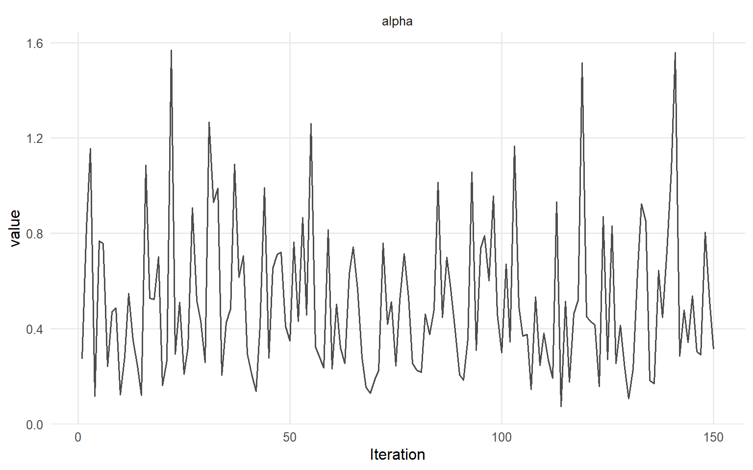
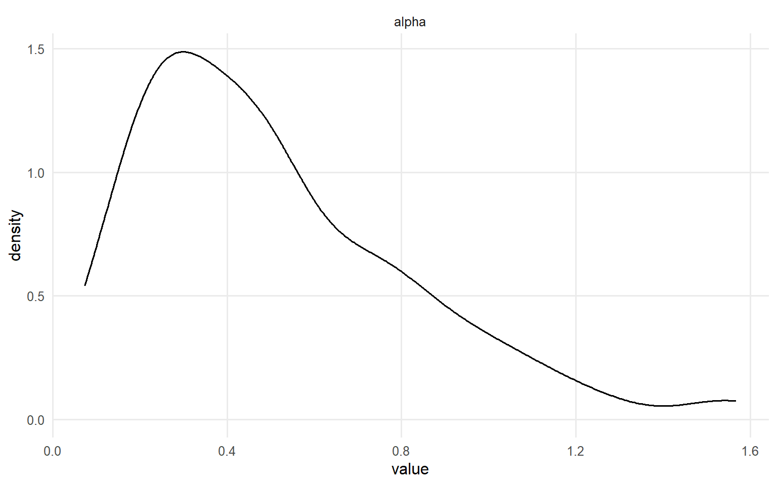
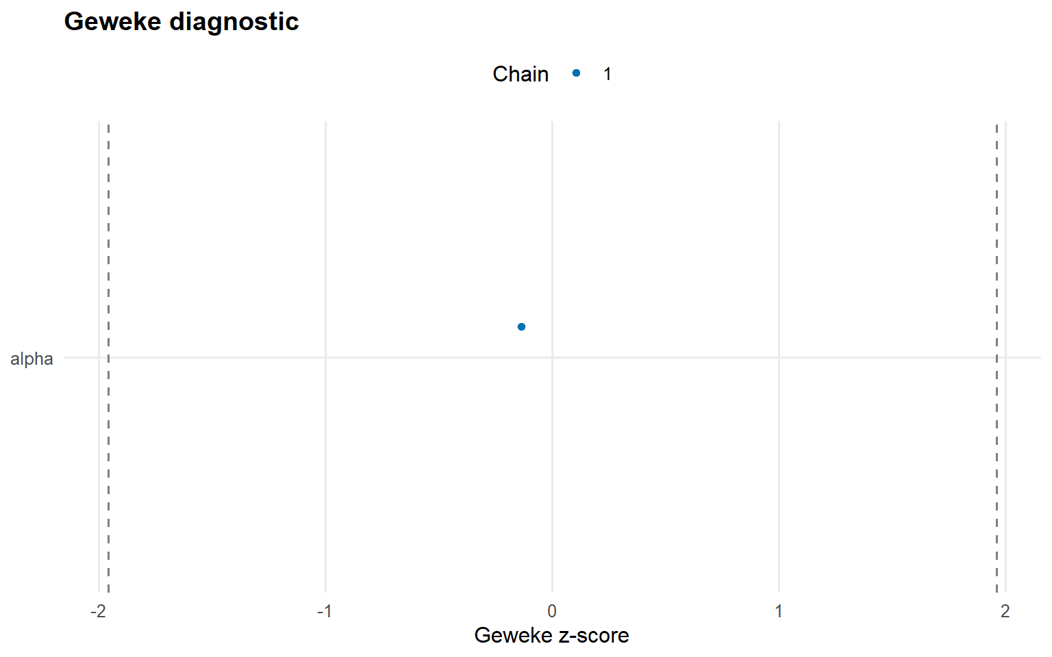
# Trace plots for key parameters
plot(fit_crp, params = "alpha", family = c("traceplot", "density", "geweke"))


=== traceplot ===


=== density ===


=== geweke ===

Posterior Predictions

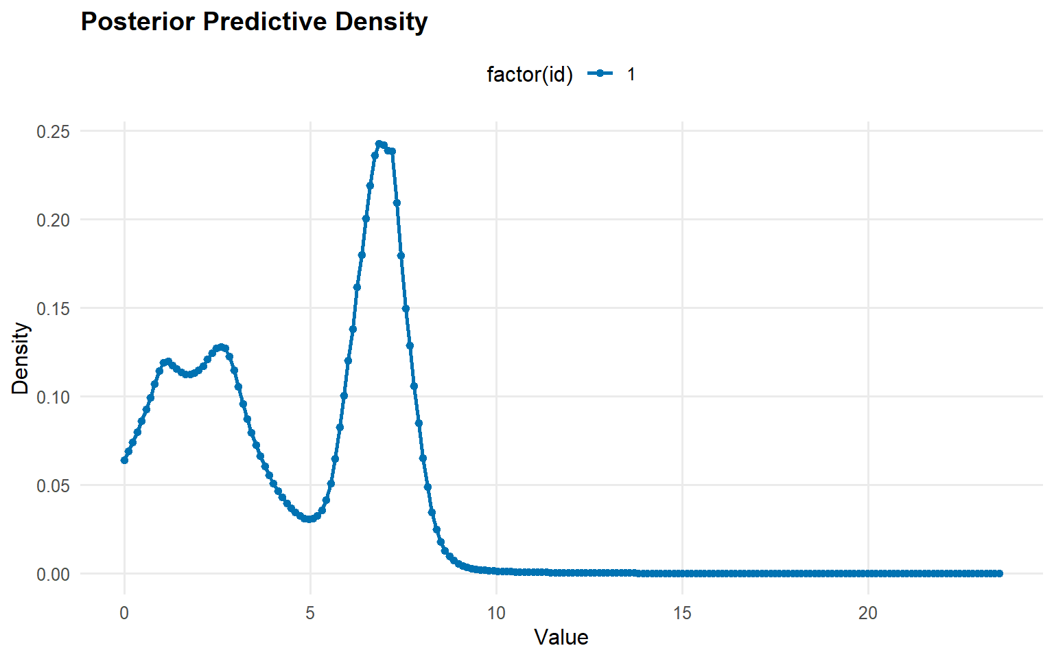
Predictive Density

Code

# Generate prediction grid
y_grid <- seq(0, max(y_mixed) * 1.2, length.out = 200)

# Posterior predictive density
pred_density <- predict(fit_crp, y = y_grid, type = "density")

# Use S3 plot method
plot(pred_density)

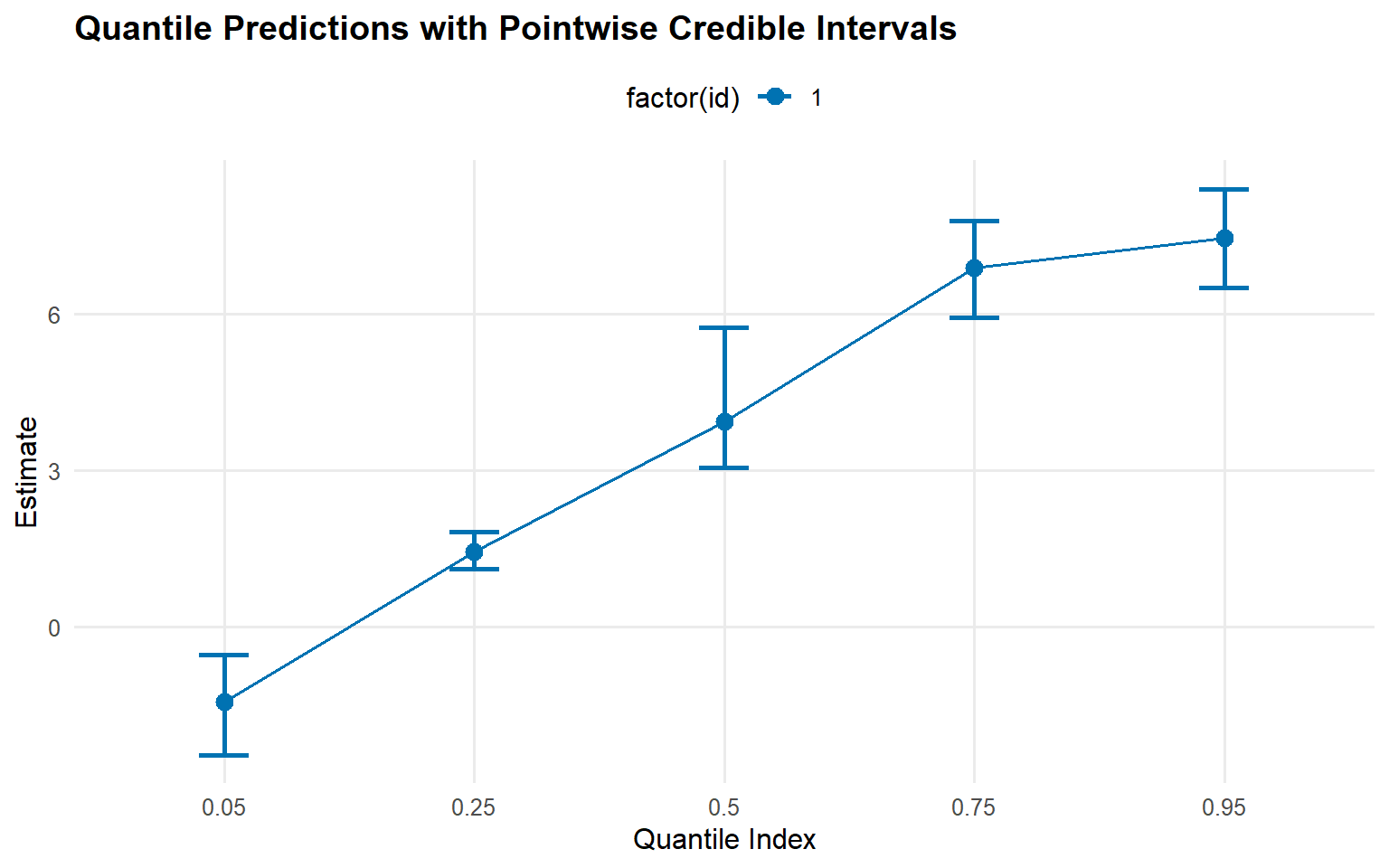
Quantile Predictions

Code

# Posterior predictive quantiles with credible intervals
quantiles_pred <- predict(fit_crp, type = "quantile", p = c(0.05, 0.25, 0.5, 0.75, 0.95),
                          interval = "credible")

# Use S3 plot method
plot(quantiles_pred)

Varying Truncation Level (components)

Code

# Demonstrate with one value
bundle_components <- bundle(
  y = y_mixed,
  kernel = "laplace",
  backend = "crp",
  components = 5,
  mcmc = mcmc
)
fit_components <- load_or_fit("ex01-unconditional-dpm-crp-fit_components", dpmix(bundle_components))

Code

summary(fit_components)

MixGPD summary | backend: Chinese Restaurant Process | kernel: Laplace Distribution | GPD tail: FALSE | epsilon: 0.025
n = 200 | components = 5
Summary
Initial components: 5 | Components after truncation: 3

WAIC: 873.554
lppd: -291.702 | pWAIC: 145.075

Summary table
   parameter  mean    sd q0.025 q0.500 q0.975    ess
  weights[1] 0.351 0.058  0.264  0.335   0.49 24.589
  weights[2] 0.268 0.042  0.195   0.27  0.346 31.995
  weights[3] 0.201 0.042   0.11    0.2  0.281   9.12
       alpha 0.808 0.442  0.183  0.722   1.78    150
 location[1]   3.2 2.543  0.803  2.349  7.961 10.681
 location[2] 4.566 3.273  0.741  2.824  9.893 11.698
 location[3] 4.393 3.496  0.423  2.691   10.3 22.648
    scale[1] 1.215 0.686  0.269  1.162  2.352 11.444
    scale[2] 1.129 0.793   0.25  1.044  2.791 22.497
    scale[3] 1.486 1.113   0.28  1.291  3.987 19.074

For unconditional models, use predict() for posterior summaries; fitted() and residuals() are not supported.

Model Comparison: Different Kernels

Laplace Kernel (Current)

Code

bundle_laplace <- bundle(
  y = y_mixed,
  kernel = "laplace",
  backend = "crp",
  components = 5,
  mcmc = mcmc
)
fit_laplace <- load_or_fit("ex01-unconditional-dpm-crp-fit_laplace", dpmix(bundle_laplace))

Code

summary(fit_laplace)

MixGPD summary | backend: Chinese Restaurant Process | kernel: Laplace Distribution | GPD tail: FALSE | epsilon: 0.025
n = 200 | components = 5
Summary
Initial components: 5 | Components after truncation: 3

WAIC: 900.436
lppd: -326.205 | pWAIC: 124.013

Summary table
   parameter  mean    sd q0.025 q0.500 q0.975     ess
  weights[1] 0.403 0.042  0.307  0.405  0.475  24.123
  weights[2] 0.323 0.052  0.229  0.325  0.411   6.766
  weights[3] 0.223 0.047  0.119  0.225  0.301  18.724
       alpha 0.755 0.431  0.178  0.654  1.752 100.851
 location[1] 6.039 2.085   1.15  6.827  7.776  37.299
 location[2] 2.794 2.148  0.795  2.305  7.416  37.024
 location[3] 1.564 1.098  0.491  1.159  2.745   13.27
    scale[1]  0.51 0.421  0.269  0.337  1.773  58.471
    scale[2] 1.284 0.585  0.313  1.274  2.392  50.835
    scale[3] 2.073 0.819  0.846  2.082  3.777  24.931

Amoroso Kernel (Alternative)

Code

bundle_amoroso <- bundle(
  y = y_mixed,
  kernel = "amoroso",
  backend = "crp",
  components = 5,
  mcmc = mcmc
)
fit_amoroso <- load_or_fit("ex01-unconditional-dpm-crp-fit_amoroso", dpmix(bundle_amoroso))

Code

summary(fit_amoroso)

MixGPD summary | backend: Chinese Restaurant Process | kernel: Amoroso Distribution | GPD tail: FALSE | epsilon: 0.025
n = 200 | components = 5
Summary
Initial components: 5 | Components after truncation: 2

WAIC: 819.477
lppd: -356.289 | pWAIC: 53.45

Summary table
  parameter   mean    sd q0.025 q0.500 q0.975    ess
 weights[1]  0.637  0.08  0.505  0.647  0.781  5.601
 weights[2]   0.35 0.082  0.204  0.345  0.485  5.217
      alpha  0.549 0.351  0.057  0.487  1.345 72.953
     loc[1] -0.002  0.22 -0.112  0.028   0.04 36.674
     loc[2]  1.774  1.34 -1.356  2.098   3.74  3.383
   scale[1]  2.931  0.52  1.629  3.022  3.749 16.876
   scale[2]  1.673 0.644   0.86  1.519  3.202   5.92
  shape1[1]  0.647 0.668  0.233  0.603  0.918 52.106
  shape1[2]   3.76 1.042  1.923  3.856  5.836   7.17
  shape2[1]  2.362 1.173  1.278  1.966  4.822   1.52
  shape2[2]  0.977 0.403  0.803  0.945  1.024 58.526

Model Comparison via Predictions

Code

# Compare models using predict() (fitted/residuals not supported for unconditional)
pred_laplace <- predict(fit_laplace, type = "mean", level = 0.9, interval = "credible")
pred_amoroso <- predict(fit_amoroso, type = "mean", level = 0.9, interval = "credible")

Code

# For unconditional models, fitted() is not supported; use predict() for comparisons (see pred_laplace, pred_amoroso above).

Key Takeaways

CRP Backend: Flexible cluster assignment, ideal for unknown mixture complexity
components Parameter: A higher components cap allows more represented mixture components but increases computation
Kernel Choice: Laplace and Amoroso illustrate two different bulk-kernel choices for the same unconditional CRP workflow
Diagnostics: Check convergence (Rhat, ESS) and posterior predictive fit
Next: Compare with Stick-Breaking (SB) backend in ex02

Prereqs

Required packages and data for this page are listed in the setup chunks above.

Outputs

This page renders model fits, diagnostics, and summary artifacts generated by package APIs.

Interpretation

Canonical concept page: Model Umbrella
Treat this page as an application/example view and use the canonical page for core definitions.

Continue to the linked canonical concept page, then return for implementation-specific details.

Unconditional DPmix: Chinese Restaurant Process (CRP)

What you’ll learn

When to use this template

Goal (in one sentence)

Data Setup

Model Specification & Bundle

Summary of MCMC Bundle

Running MCMC

Summary of Fitted MCMC model

MCMC Diagnostics Plots

Posterior Predictions

Predictive Density

Quantile Predictions

Varying Truncation Level (components)

Model Comparison: Different Kernels

Laplace Kernel (Current)

Amoroso Kernel (Alternative)

Model Comparison via Predictions

Key Takeaways

Workflow Navigation

Prereqs

Outputs

Interpretation

Next