ex02. Unconditional DPM (SB Backend)

Website workflow note. This page reflects the current exported API and recommended wrapper-first usage. Last updated: 2026-02-19.

For the full package narrative, see the main package vignettes (basic, unconditional, conditional, and causal).

Unconditional DPmix: Stick-Breaking (SB) Backend

Purpose: Showcase the stick-breaking backend that uses a fixed number of mixture components (components = J) and contrast it with the CRP backend from start/backends-and-workflow. In this vignette we fit two bulk kernels (Gamma and Cauchy) on the same dataset to highlight how heavier tails in the bulk can change the fit even without a GPD tail.

What you’ll learn

How the stick-breaking (SB) backend differs from CRP in practice (fixed truncation via components = J).
How to use bundle() + dpmix() + predict()/plot() for an unconditional bulk-only DP mixture.
How bulk kernel choice (e.g., Gamma vs Cauchy) can change tail behavior even when GPD = FALSE.

When to use this template

You want a predictable runtime mixture workflow with a fixed upper bound on components.
You mainly care about bulk fit, density estimation, and posterior predictive summaries.

Next steps

If extremes matter, extend to dpmgpd() with GPD = TRUE (see ex03/ex04).

Data Setup

Code

# Generate a reproducible mock dataset instead of relying on saved cache files.
set.seed(10102)
n <- 200
weights <- c(0.4, 0.35, 0.25)
params <- list(
  list(shape = 2.0, rate = 1.5),
  list(shape = 4.0, rate = 1.0),
  list(shape = 7.0, rate = 0.7)
)
component <- sample(seq_along(weights), size = n, replace = TRUE, prob = weights)
y_mixed <- numeric(n)
for (k in seq_along(params)) {
  idx <- which(component == k)
  if (length(idx) > 0) {
    y_mixed[idx] <- rgamma(length(idx), shape = params[[k]]$shape, rate = params[[k]]$rate)
  }
}

df_data <- data.frame(y = y_mixed)

summary_tbl <- tibble(
  statistic = c("N", "Mean", "SD", "Min", "Max"),
  value = c(length(y_mixed), mean(y_mixed), sd(y_mixed), min(y_mixed), max(y_mixed))
)

p_raw <- ggplot(df_data, aes(x = y)) +
  geom_histogram(aes(y = after_stat(density)), bins = 30, fill = "darkorange", alpha = 0.7, color = "black") +
  geom_density(color = "darkred", linewidth = 1.2) +
  labs(title = "Raw Data: Mixed Gamma Distribution", x = "y", y = "Density") +
  theme_minimal()

print(p_raw)

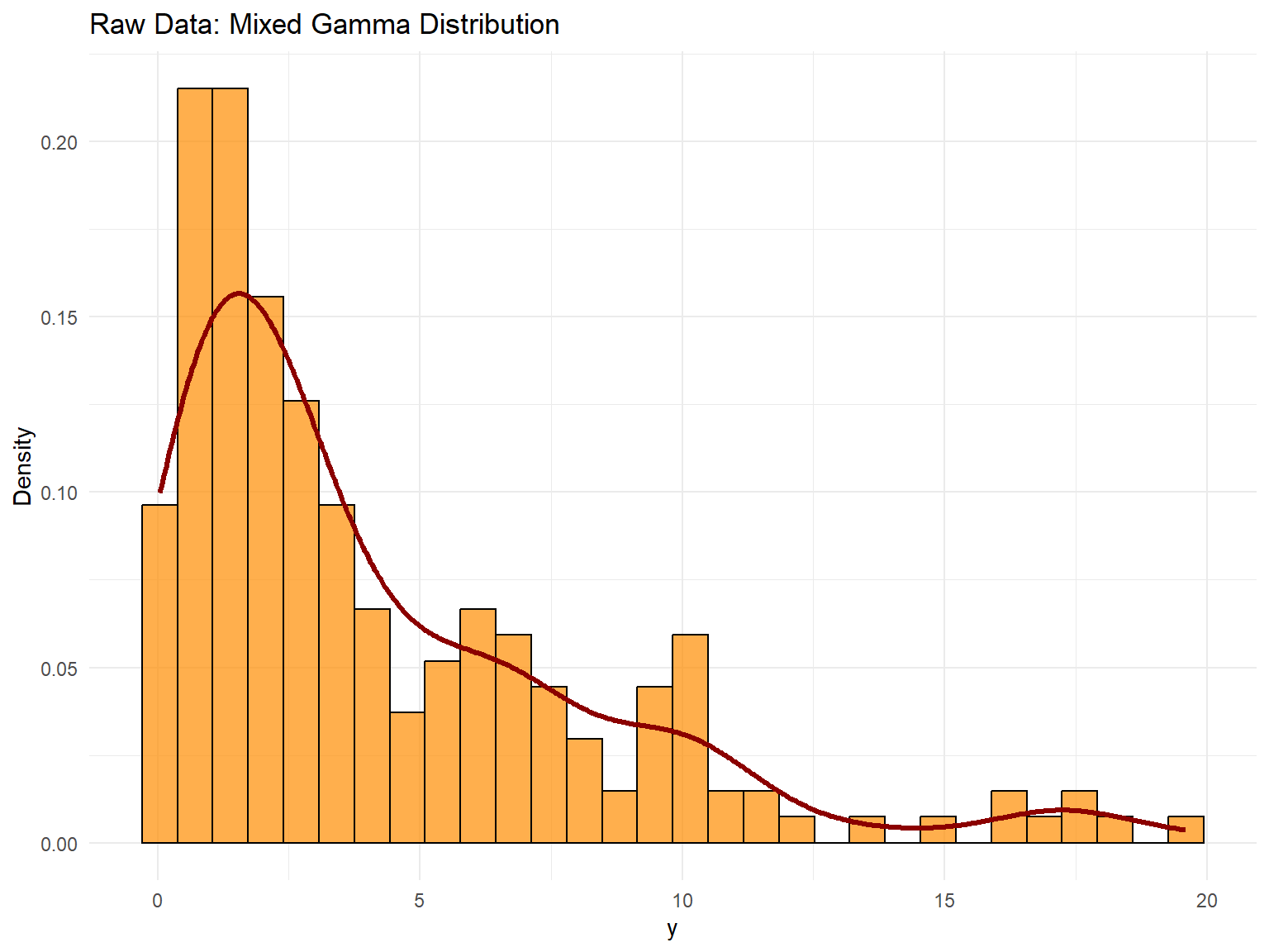
# A tibble: 5 × 2
  statistic    value
  <chr>        <dbl>
1 N         200     
2 Mean        4.21  
3 SD          4.11  
4 Min         0.0403
5 Max        19.6

Model Specification & Bundle

We build the stick-breaking mixture explicitly with components = 5 so that there is room for weight decay while keeping the MCMC runtime manageable for a vignette. We then refit the same SB model with a Cauchy kernel for comparison.

Code

# --- Gamma kernel ---
bundle_sb_gamma <- bundle(
  y = y_mixed,
  kernel = "gamma",
  backend = "sb",
  components = 5,            # fixed truncation level for SB
  GPD = FALSE,               # bulk-only scenario
  mcmc = mcmc
)

# --- Cauchy kernel ---
bundle_sb_cauchy <- bundle(
  y = y_mixed,
  kernel = "cauchy",
  backend = "sb",
  components = 5,
  GPD = FALSE,
  mcmc = mcmc
)

Running MCMC & Summary

Code

fit_sb_gamma <- load_or_fit("ex02-unconditional-dpm-sb-fit_sb_gamma", dpmix(bundle_sb_gamma))
fit_sb_cauchy <- load_or_fit("ex02-unconditional-dpm-sb-fit_sb_cauchy", dpmix(bundle_sb_cauchy))

Code

summary(fit_sb_gamma)

MixGPD summary | backend: Stick-Breaking Process | kernel: Gamma Distribution | GPD tail: FALSE | epsilon: 0.025
n = 200 | components = 5
Summary
Initial components: 5 | Components after truncation: 3

Summary table
  parameter  mean    sd q0.025 q0.500 q0.975    ess
 weights[1] 0.395 0.042  0.334  0.387  0.485  3.212
 weights[2] 0.321 0.035  0.242  0.323  0.393 17.083
 weights[3] 0.195  0.05  0.108  0.202   0.28  7.824
      alpha 1.186 0.609  0.305  1.083  2.407 44.491
   shape[1] 2.237 1.283  1.025   1.55  4.779 10.926
   shape[2] 3.462  1.43  1.138  3.483  5.654  7.937
   shape[3] 2.602 1.228  1.226  2.204  5.166  8.559
   scale[1] 0.575 0.194   0.32  0.571  0.896 28.382
   scale[2] 0.773 0.555  0.293  0.571  2.199  4.083
   scale[3] 1.224 0.589  0.399   1.12  2.446  7.623

Code

summary(fit_sb_cauchy)

MixGPD summary | backend: Stick-Breaking Process | kernel: Cauchy Distribution | GPD tail: FALSE | epsilon: 0.025
n = 200 | components = 5
Summary
Initial components: 5 | Components after truncation: 3

Summary table
   parameter  mean    sd q0.025 q0.500 q0.975    ess
  weights[1] 0.502 0.081  0.378  0.481  0.621  3.202
  weights[2] 0.232 0.035  0.169  0.232  0.315 19.143
  weights[3] 0.147 0.044  0.064   0.16  0.212  5.279
       alpha  1.32 0.645  0.321  1.272  2.743 52.126
 location[1]  1.25 0.182  0.995    1.2  1.569  5.851
 location[2] 5.649 2.556  2.646  5.997  9.852  8.551
 location[3]   5.2 2.037  2.534  5.446  9.832 34.878
    scale[1] 0.637 0.139  0.431  0.617  0.912 11.565
    scale[2] 1.312  0.72  0.473   1.07  2.923 14.081
    scale[3] 1.058  0.52  0.367  1.003  2.341 76.149

Code

params_gamma <- params(fit_sb_gamma)
params_gamma

Posterior mean parameters

$alpha
[1] 1.186

$w
[1] 0.3947 0.3213 0.1948

$shape
[1] 2.237 3.462 2.602

$scale
[1] 0.5752 0.7728 1.2240

MCMC Diagnostics (S3 Plot Methods)

Code

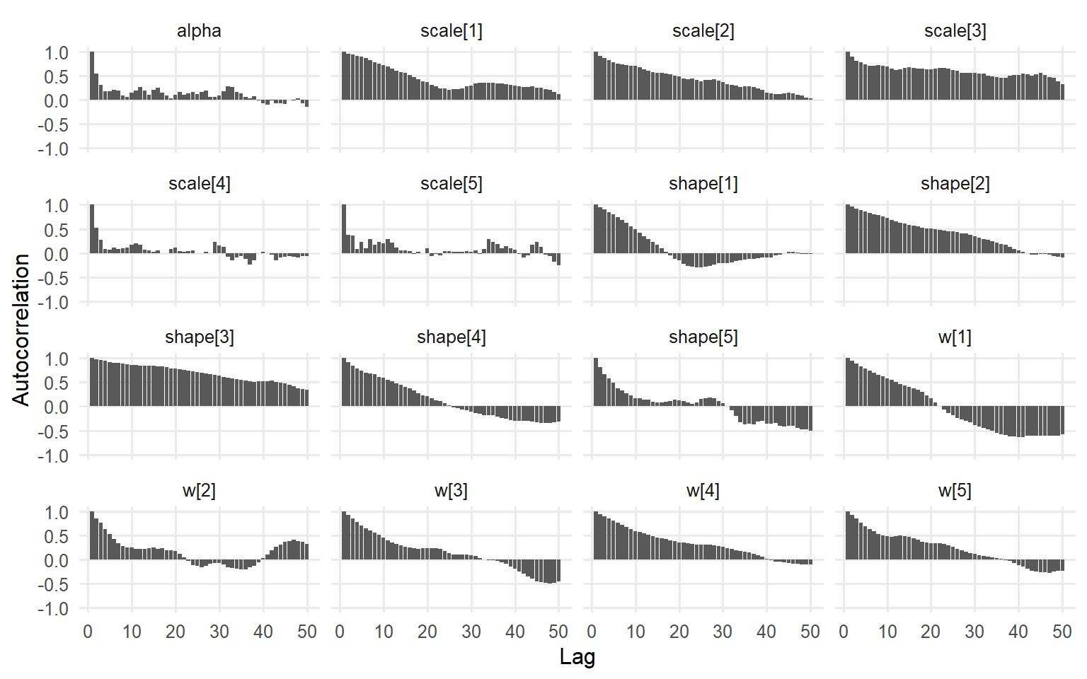
# Default diagnostics for each fit
plot(fit_sb_gamma, family = c("traceplot", "autocorrelation", "running"))


=== traceplot ===


=== autocorrelation ===


=== running ===

Code

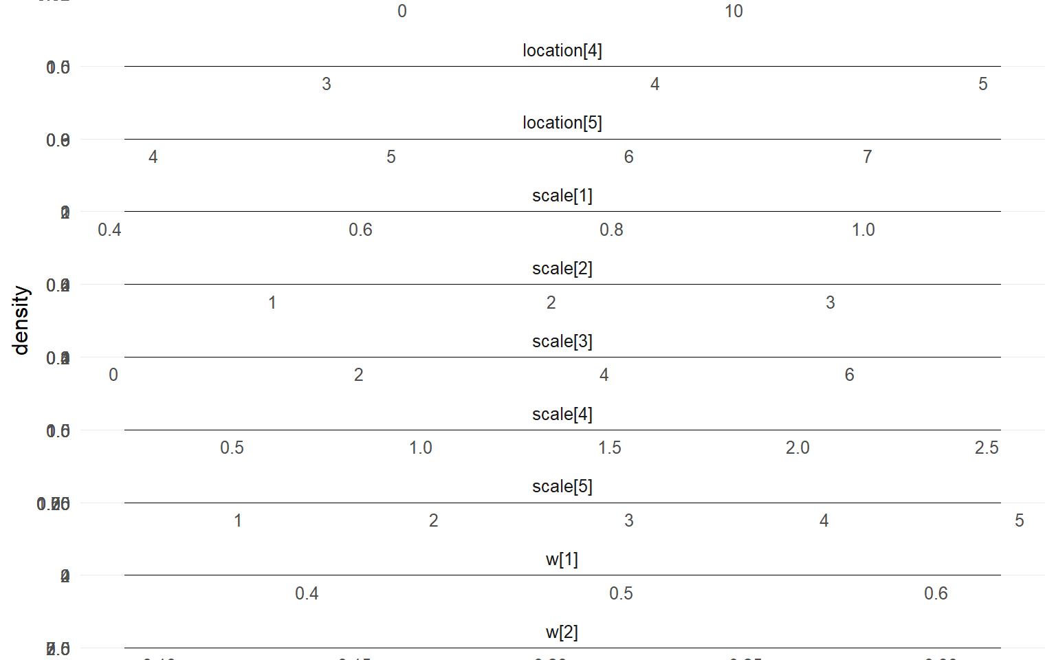
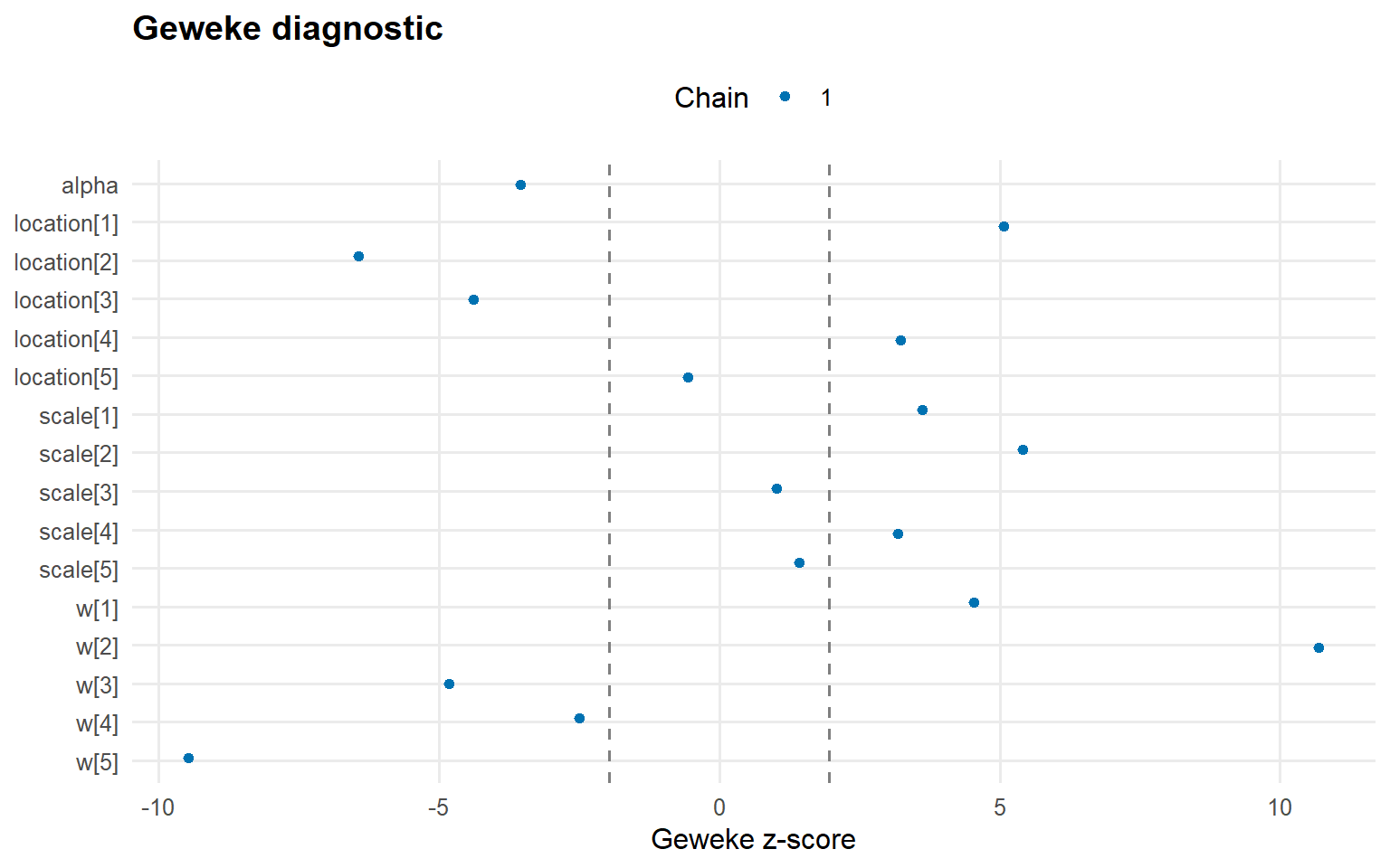
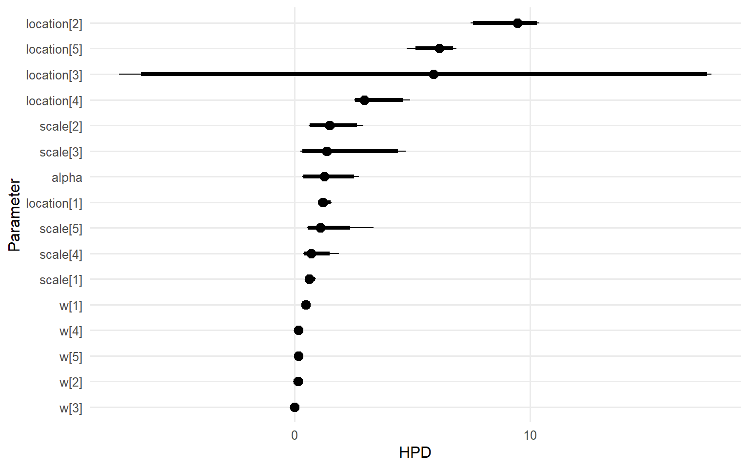
plot(fit_sb_cauchy, family = c("density", "geweke", "caterpillar"))


=== density ===


=== geweke ===


=== caterpillar ===

Use summary(fit_sb_gamma) and summary(fit_sb_cauchy) to inspect effective sample size, R-hat, and other convergence diagnostics; the plot() calls above show the trace/density pairs for both global and stick-breaking weight parameters.

Stick-Breaking Weights & Component Activity

The stick-breaking weights are exposed via the plot() diagnostics above, and you can refer to the raw fit_sb_gamma / fit_sb_cauchy objects (or their summary() output) for posterior summaries of each component weight.

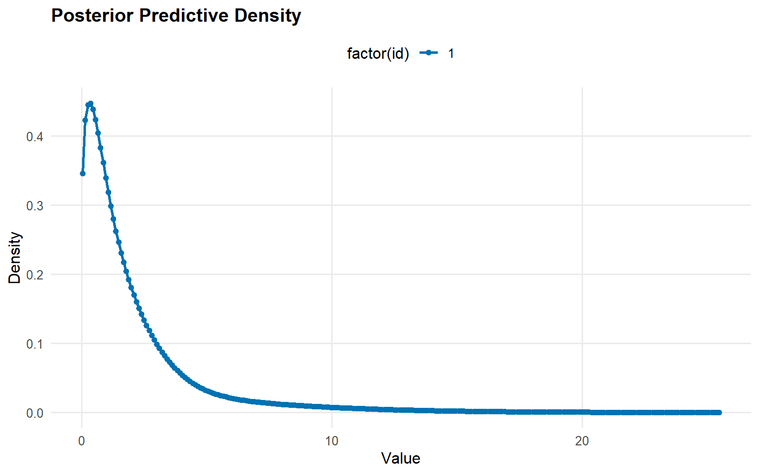
Posterior Predictions

Code

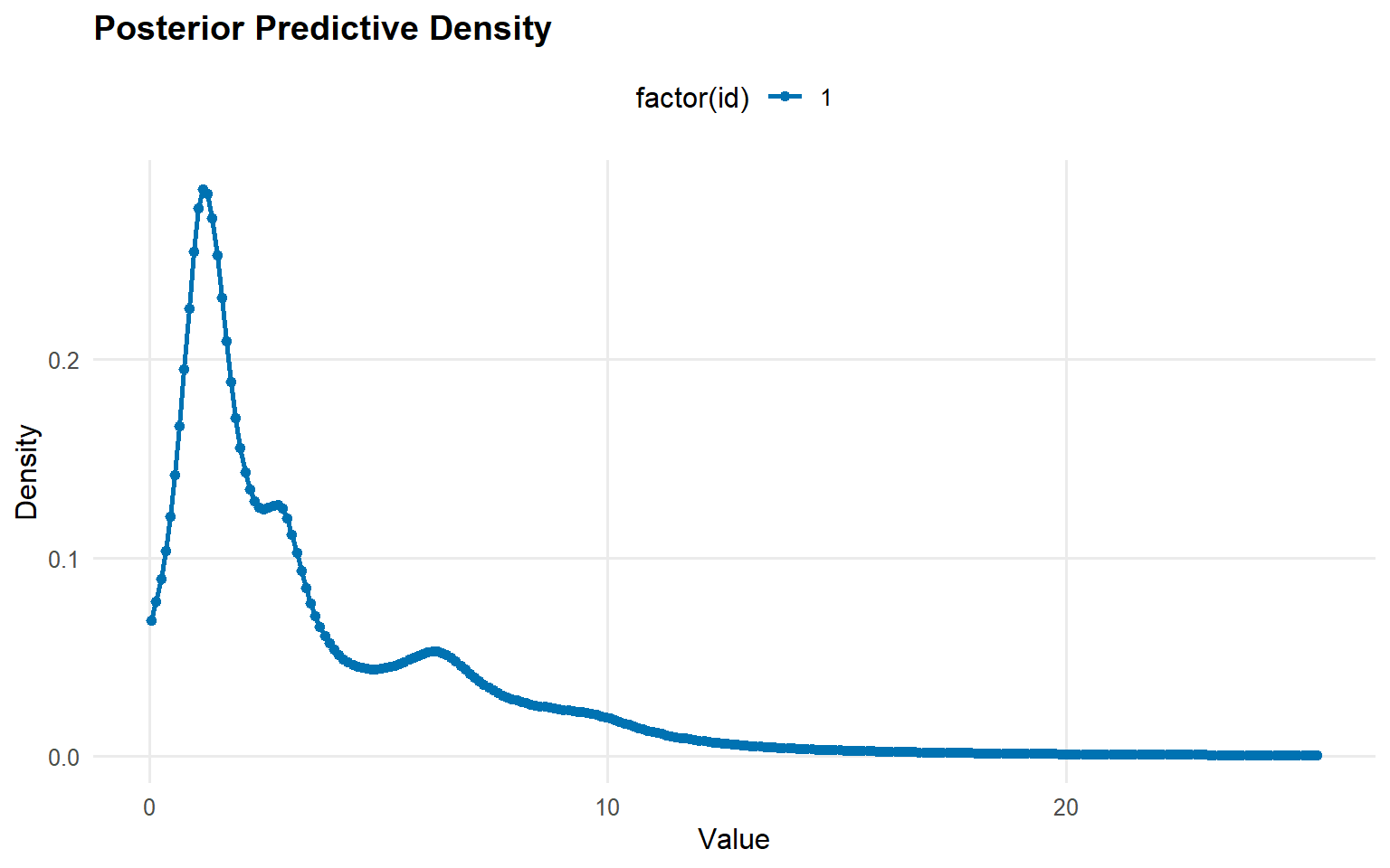
y_grid <- seq(min(y_mixed), max(y_mixed) * 1.3, length.out = 250)

pred_density_gamma <- predict(fit_sb_gamma, y = y_grid, type = "density")
pred_density_cauchy <- predict(fit_sb_cauchy, y = y_grid, type = "density")

plot(pred_density_gamma)

Code

plot(pred_density_cauchy)

Code

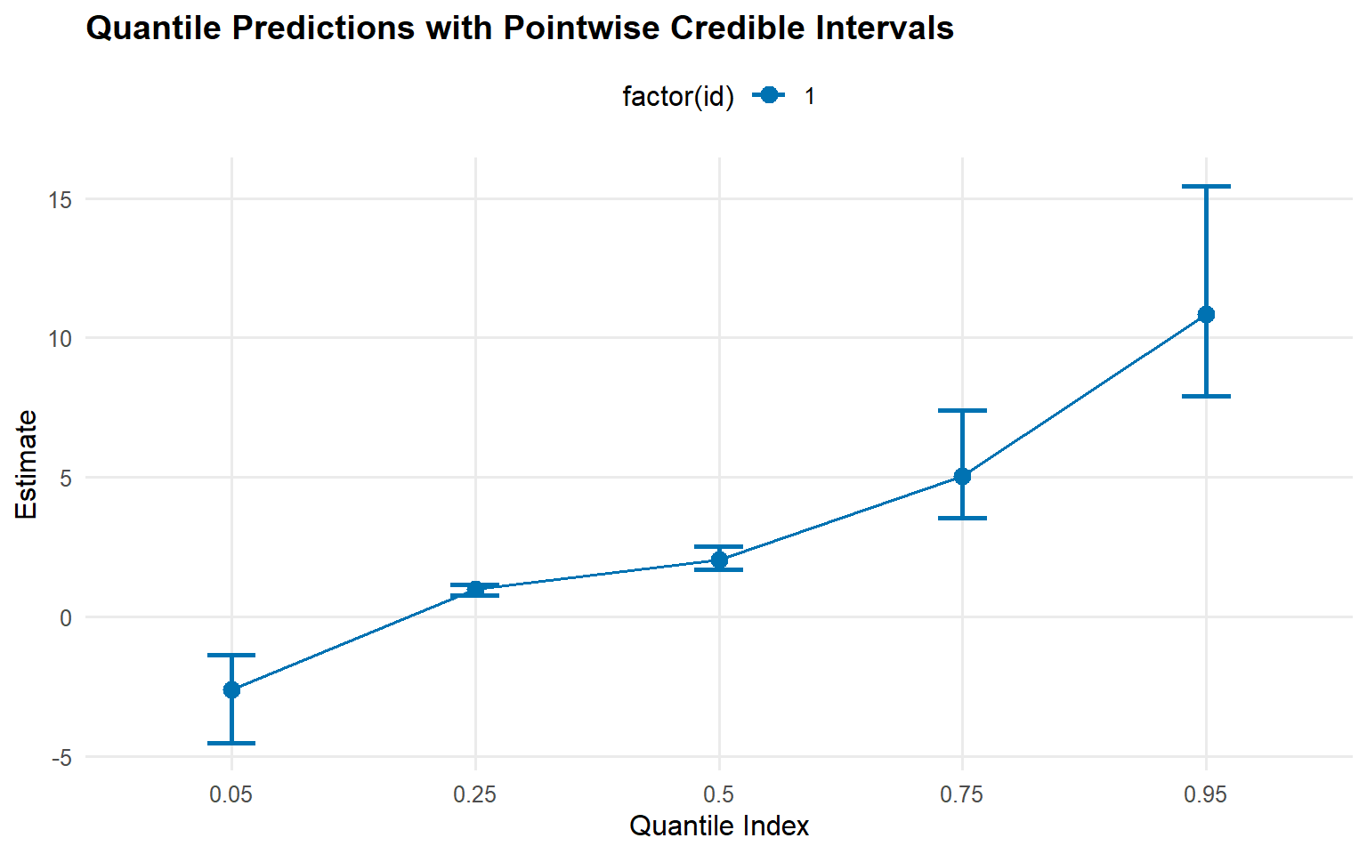
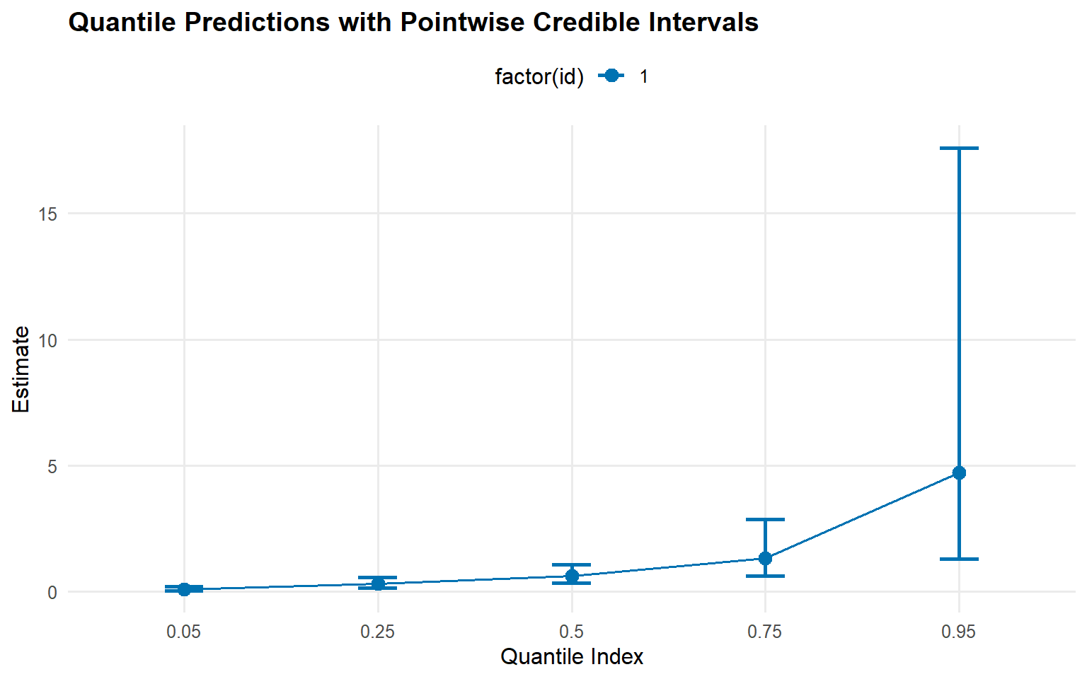
quant_probs <- c(0.05, 0.25, 0.5, 0.75, 0.95)

pred_q_gamma <- predict(fit_sb_gamma, type = "quantile", p = quant_probs, interval = "credible")
pred_q_cauchy <- predict(fit_sb_cauchy, type = "quantile", p = quant_probs, interval = "credible")

plot(pred_q_gamma)

Code

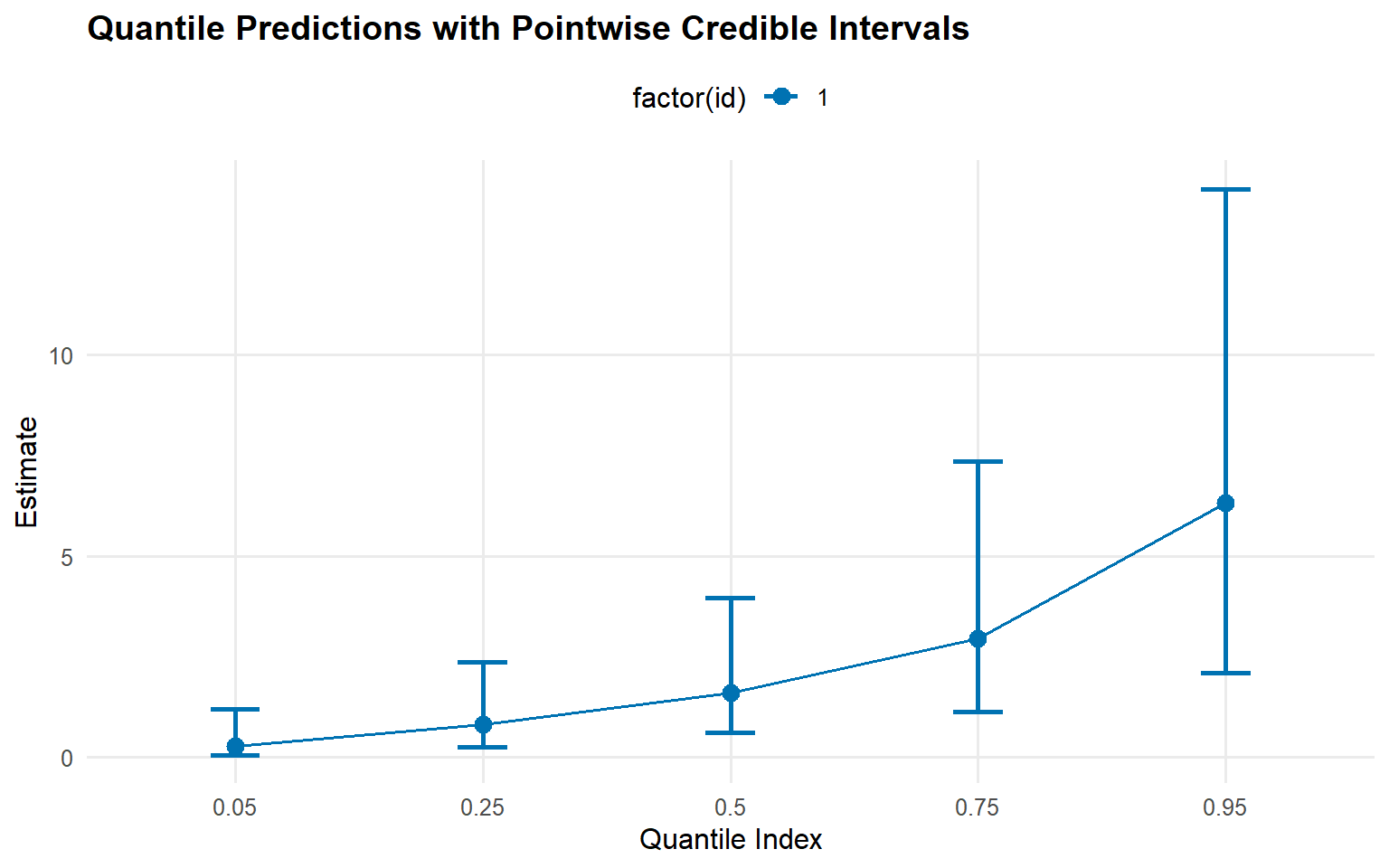
plot(pred_q_cauchy)

Code

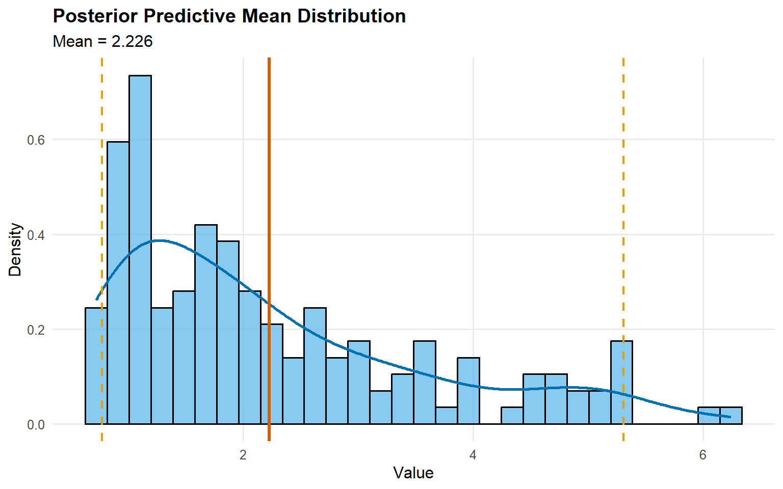
pred_mean_gamma <- predict(fit_sb_gamma, type = "mean")
pred_mean_cauchy <- predict(fit_sb_cauchy, type = "mean")

plot(pred_mean_gamma)

Code

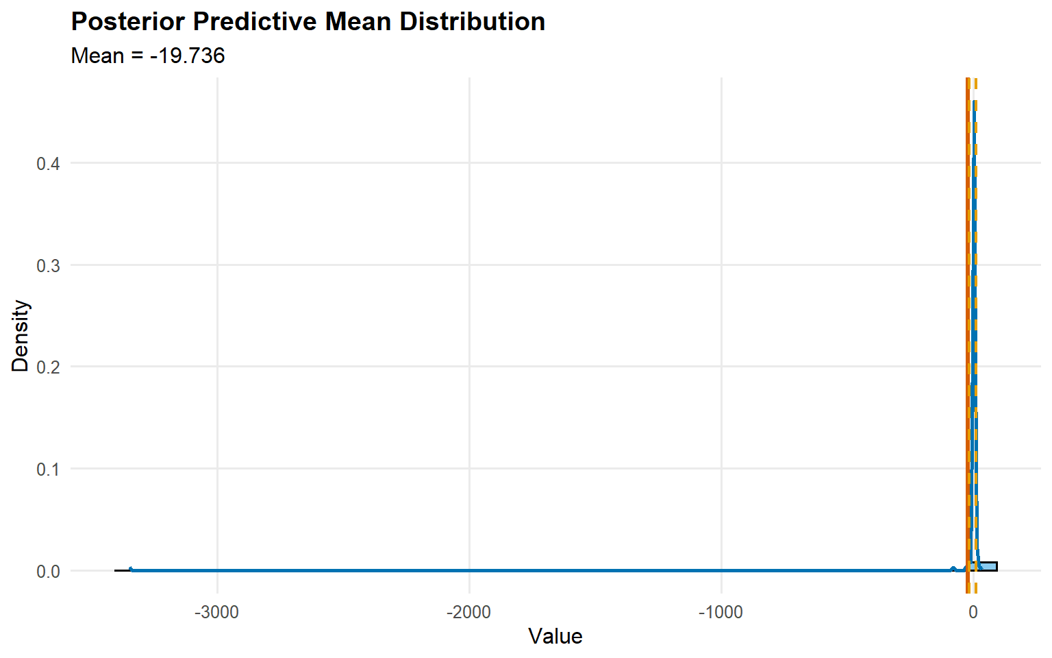
plot(pred_mean_cauchy)

Bulk-only vs CRP Backends

Code

bundle_crp_small <- bundle(
  y = y_mixed,
  kernel = "gamma",
  backend = "crp",
  components = 5,
  GPD = FALSE,
  mcmc = mcmc
)
fit_crp_small <- load_or_fit("ex02-unconditional-dpm-sb-fit_crp_small", dpmix(bundle_crp_small))

crp_quant <- predict(fit_crp_small, type = "quantile", p = quant_probs, interval = "credible")
sb_quant <- predict(fit_sb_gamma, type = "quantile", p = quant_probs, interval = "credible")

bind_rows(
  crp_quant$fit %>% mutate(model = "CRP"),
  sb_quant$fit %>% mutate(model = "SB")
) %>%
  select(any_of(c("model", "index", "estimate", "lower", "upper")))

   model index  estimate      lower     upper
1    CRP  0.05 0.1067670 0.04176633  0.213226
2    CRP  0.25 0.3266968 0.16551984  0.568718
3    CRP  0.50 0.6314040 0.34692305  1.082989
4    CRP  0.75 1.3282693 0.62991581  2.862594
5    CRP  0.95 4.7332026 1.30743509 17.604264
6     SB  0.05 0.2686400 0.04578688  1.181490
7     SB  0.25 0.8059203 0.24201029  2.351381
8     SB  0.50 1.6058160 0.59798532  3.955477
9     SB  0.75 2.9409217 1.13342608  7.342066
10    SB  0.95 6.3086670 2.08820530 14.132008

Code

plot(crp_quant)

Code

plot(sb_quant)

For unconditional models, use predict() only; fitted() and residuals() are not supported.

Takeaways

SB Backend: Fixed components keeps label-switching manageable, and the diagnostic plots via the S3 plot() method show weight dynamics.
Kernels matter: Gamma vs Cauchy can behave very differently in the shoulders/tails, even without a GPD tail.
Predictions: Posterior density, posterior-mean quantiles, and mean (via predictive sampling) are accessible via predict() with pointwise 95% credible intervals.
Backend comparison: The CRP fit (start/backends-and-workflow) and the SB-gamma fit deliver similar central quantiles while SB offers more control over truncation.
Next: Explore tail augmentation (GPD = TRUE) with the CRP backend in ex03 or SB backend in ex04.

Prereqs

Required packages and data for this page are listed in the setup chunks above.

Outputs

This page renders model fits, diagnostics, and summary artifacts generated by package APIs.

Interpretation

Canonical concept page: Model Umbrella
Treat this page as an application/example view and use the canonical page for core definitions.

Continue to the linked canonical concept page, then return for implementation-specific details.

Unconditional DPmix: Stick-Breaking (SB) Backend

What you’ll learn

When to use this template

Next steps

Data Setup

Model Specification & Bundle

Running MCMC & Summary

MCMC Diagnostics (S3 Plot Methods)

Stick-Breaking Weights & Component Activity

Posterior Predictions

Bulk-only vs CRP Backends

Takeaways

Workflow Navigation

Prereqs

Outputs

Interpretation

Next