ex03. Unconditional DPMGPD (CRP Backend)

Website workflow note. This page reflects the current exported API and recommended wrapper-first usage. Last updated: 2026-02-19.

For the full package narrative, see the main package vignettes (basic, unconditional, conditional, and causal).

Unconditional CausalMixGPD: CRP Backend with Tail Augmentation

Purpose: Model the bulk of the distribution with a DP mixture (the “kernel” or bulk family) and let a GPD tail capture extreme values beyond a threshold. The CRP backend handles partitioning and we toggle GPD = TRUE to augment the tail.

What you’ll learn

How a bulk DP mixture + GPD tail splits modeling responsibility across typical and extreme values.
How to encode threshold behavior via param_specs and then evaluate tail summaries via predict().
How to read tail-aware predictions: density, survival, and high quantiles.

When to use this template

You have a single outcome with a visible right tail and need explicit extreme-tail modeling.
You care about tail risk summaries (survival probabilities, high quantiles), not only mean/density.

Next steps

Compare against the SB+GPD analogue (ex04) to see how truncation and partition behavior affect uncertainty.

Data Setup

Code

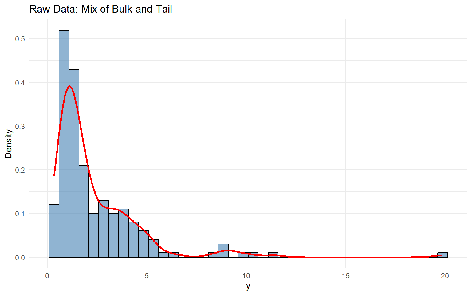
# Load data with an obvious tail
data("nc_pos_tail200_k4")
y_tail <- nc_pos_tail200_k4$y
y_tail <- y_tail[is.finite(y_tail) & y_tail > 0]

# Summaries and table
summary_tbl <- tibble(
  statistic = c("N", "Mean", "SD", "Min", "Max"),
  value = c(length(y_tail), mean(y_tail), sd(y_tail), min(y_tail), max(y_tail))
)

df_data <- data.frame(y = y_tail)

ggplot(df_data, aes(x = y)) +
  geom_histogram(aes(y = after_stat(density)), bins = 40, fill = "steelblue", color = "black", alpha = 0.6) +
  geom_density(color = "red", linewidth = 1) +
  labs(title = "Raw Data: Mix of Bulk and Tail", x = "y", y = "Density") +
  theme_minimal()

Code

summary_tbl

# A tibble: 5 × 2
  statistic   value
  <chr>       <dbl>
1 N         200    
2 Mean        2.33 
3 SD          2.30 
4 Min         0.328
5 Max        19.9

Threshold & Tail Partition

Code

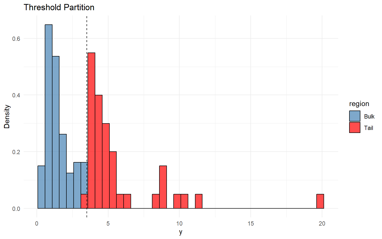
thresholds <- quantile(y_tail, c(0.70, 0.75, 0.80, 0.85, 0.90))
u_threshold <- thresholds["80%"]

df_tail <- tibble(
  y = y_tail,
  region = ifelse(y_tail > u_threshold, "Tail", "Bulk")
)

ggplot(df_tail, aes(x = y, fill = region)) +
  geom_histogram(aes(y = after_stat(density)), bins = 40, alpha = 0.7, color = "black") +
  geom_vline(xintercept = u_threshold, linetype = "dashed", color = "black") +
  scale_fill_manual(values = c("Bulk" = "steelblue", "Tail" = "red")) +
  labs(title = "Threshold Partition", x = "y", y = "Density") +
  theme_minimal()

Model Specification & Bundle

This mirrors the direct bundle() workflow in start/backends-and-workflow, but with tail augmentation turned on (GPD = TRUE). Here we use an Inverse Gaussian bulk kernel and estimate the GPD threshold with a lognormal prior centered at the empirical 80th percentile.

Code

bundle_gpd <- bundle(
  y = y_tail,
  kernel = "invgauss",
  backend = "crp",
  GPD = TRUE,
  components = 5,
  alpha_random = TRUE,
  param_specs = list(
    gpd = list(
      threshold = list(
        mode = "dist",
        dist = "lognormal",
        args = list(meanlog = log(max(u_threshold, .Machine$double.eps)), sdlog = 0.25)
      )
    )
  ),
  mcmc = mcmc
)

Running MCMC & Diagnostics

Code

fit_gpd <- load_or_fit("ex03-unconditional-dpmgpd-crp-fit_gpd", dpmgpd(bundle_gpd))

Code

summary(fit_gpd)

MixGPD summary | backend: Chinese Restaurant Process | kernel: Inverse Gaussian Distribution | GPD tail: TRUE | epsilon: 0.025
n = 200 | components = 5
Summary
Initial components: 5 | Components after truncation: 1

WAIC: 663.412
lppd: -315.476 | pWAIC: 16.23

Summary table
  parameter  mean    sd q0.025 q0.500 q0.975    ess
 weights[1] 0.904 0.165   0.51      1      1  2.748
      alpha 0.255 0.254  0.012  0.179  0.975 72.018
 tail_scale 2.413  1.11  1.184  2.087  5.329 12.461
 tail_shape 0.138 0.143 -0.185  0.124  0.422 23.417
  threshold 3.634 1.325  1.695  3.461   6.21  6.927
    mean[1] 2.382 0.551  1.197  2.284  3.858 18.962
   shape[1] 3.425 0.612  2.682   3.29  4.616 11.482

Code

params_gpd <- params(fit_gpd)
params_gpd

Posterior mean parameters

$alpha
[1] 0.255

$w
[1] 0.9045

$mean
[1] 2.382

$shape
[1] 3.425

$tail_scale
[1] 2.413

$tail_shape
[1] 0.138

Code

# S3 plot methods highlight trace + density diagnostics
plot(fit_gpd, family = c("traceplot", "density", "running"))


=== traceplot ===


=== density ===


=== running ===

Code

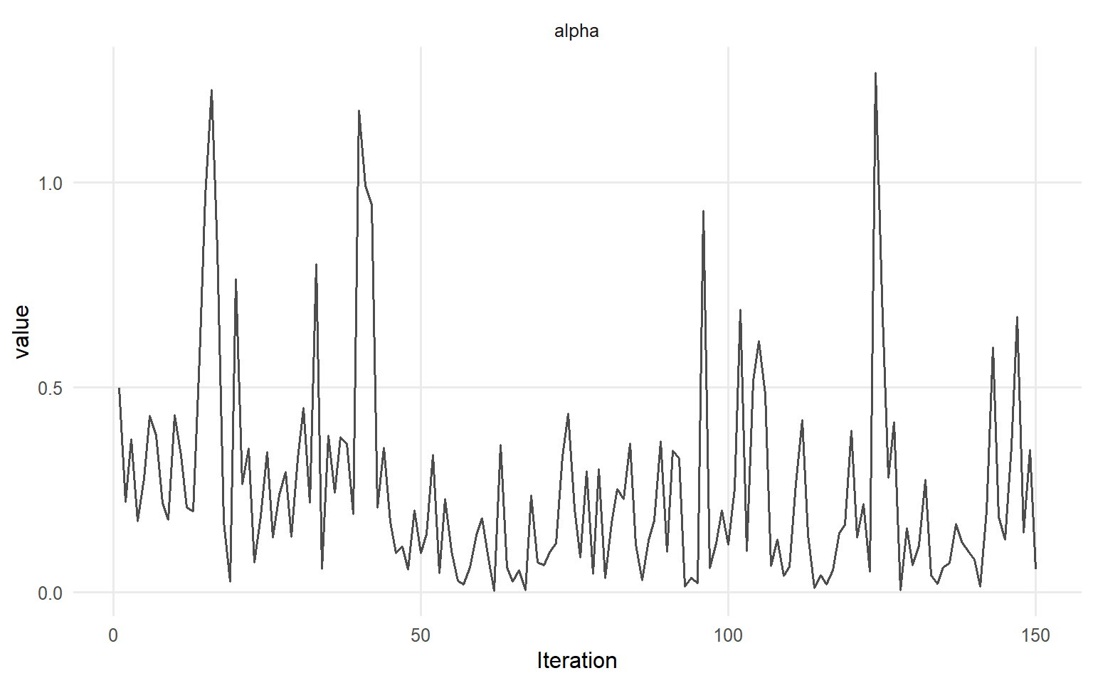
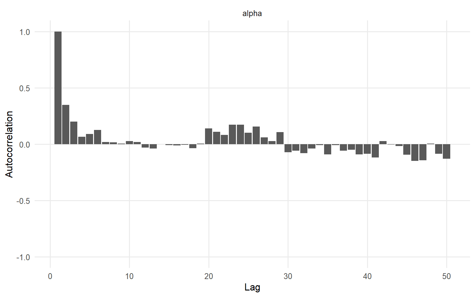
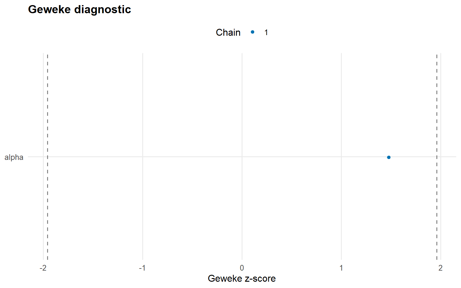
plot(fit_gpd, params = "alpha", family = c("traceplot", "autocorrelation", "geweke"))


=== traceplot ===


=== autocorrelation ===


=== geweke ===

Posterior Predictions: Bulk and Tail

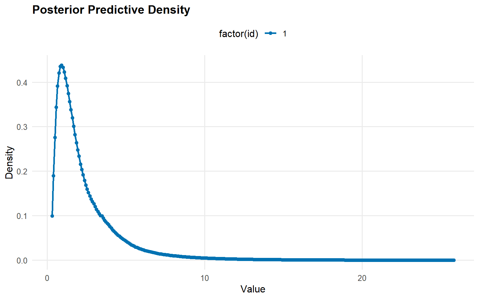
We use the S3 predict() objects and their dedicated plot() methods to visualize densities, survival curves, and posterior-mean quantiles (i.e., averages of q(p | \(\\theta\)) over draws).

Code

y_min <- max(min(y_tail), .Machine$double.eps)
y_grid <- seq(y_min, max(y_tail) * 1.3, length.out = 300)
pred_density <- predict(fit_gpd, y = y_grid, type = "density")
plot(pred_density)

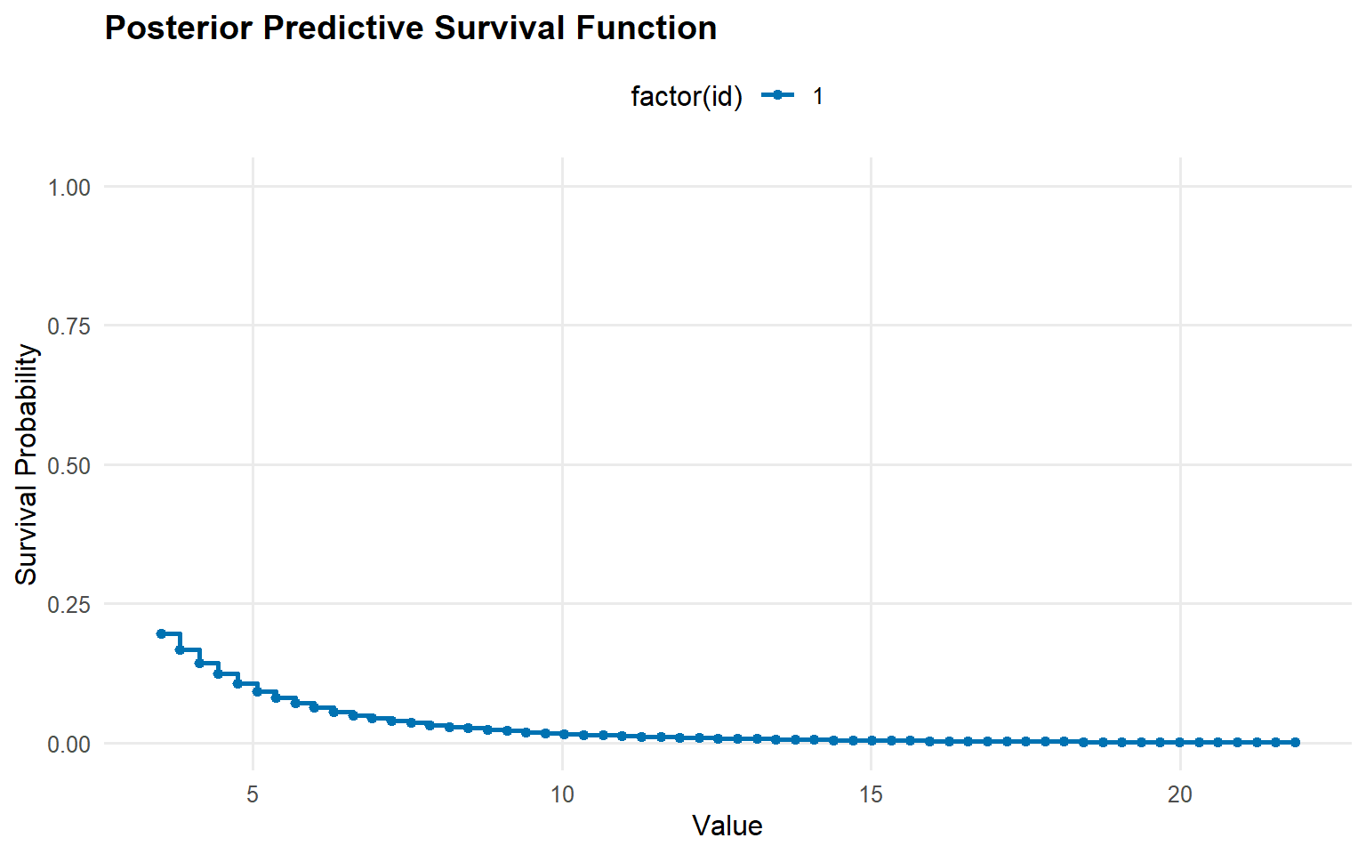
Code

y_surv <- seq(max(u_threshold, y_min), max(y_tail) * 1.1, length.out = 60)
pred_surv <- predict(fit_gpd, y = y_surv, type = "survival")
plot(pred_surv)

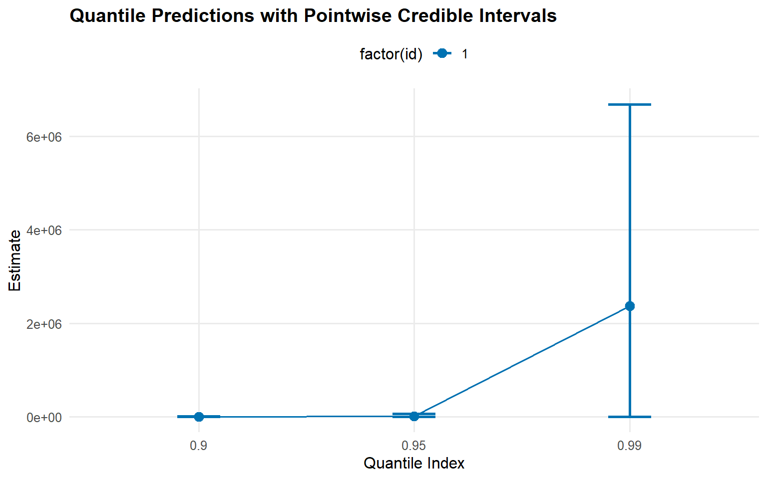
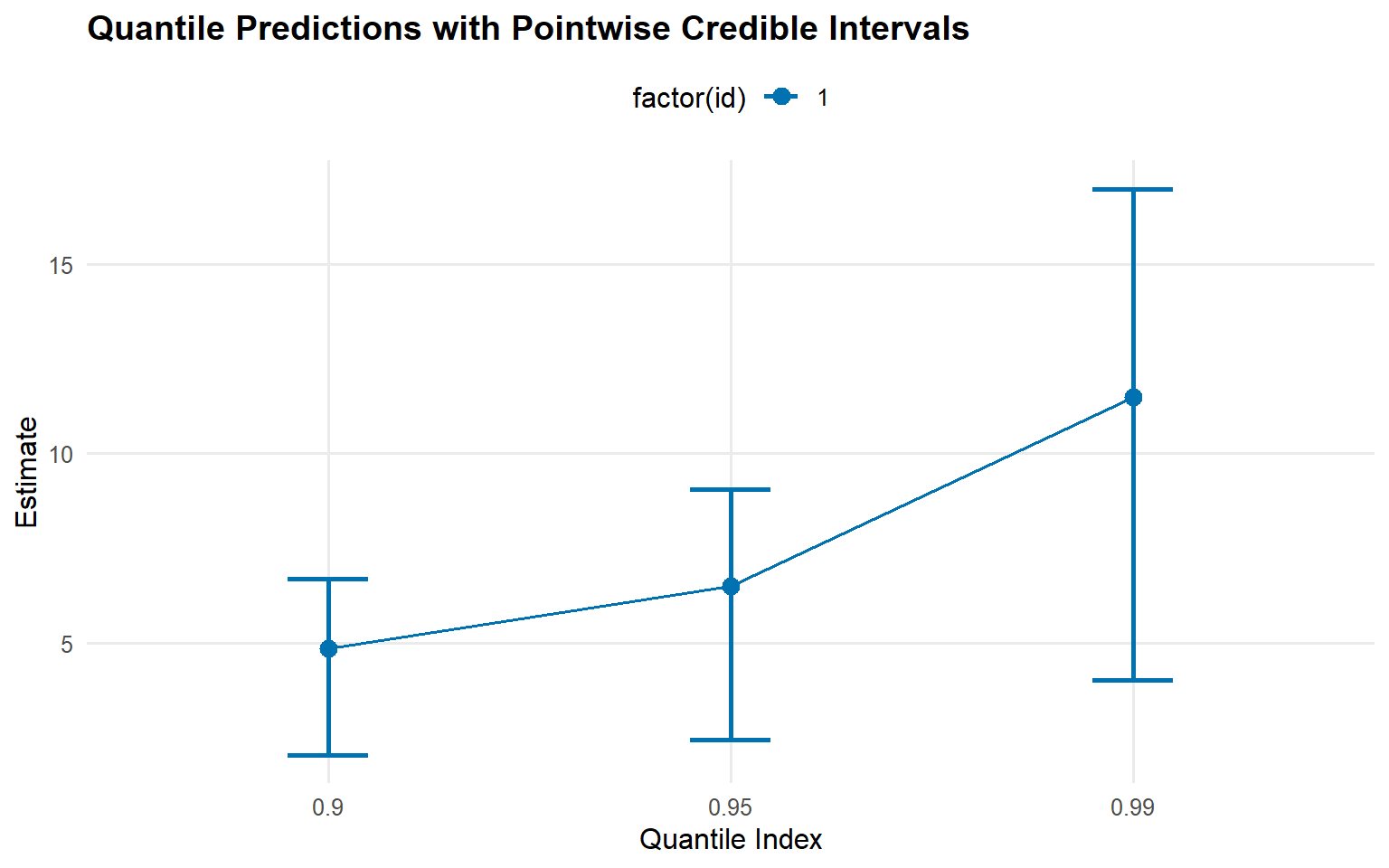
Code

quantile_probs <- c(0.90, 0.95, 0.99)
pred_quantiles <- predict(fit_gpd, type = "quantile", p = quantile_probs, interval = "credible")
plot(pred_quantiles)

Bulk-Only Baseline Comparison

To demonstrate the value of tail augmentation, we fit a bulk-only lognormal DP mixture and compare posterior summaries against the InvGauss+GPD fit.

Code

bundle_bulk_only <- bundle(
  y = y_tail,
  kernel = "lognormal",
  backend = "crp",
  GPD = FALSE,
  components = 5,
  mcmc = mcmc
)
fit_bulk_only <- load_or_fit("ex03-unconditional-dpmgpd-crp-fit_bulk_only", dpmix(bundle_bulk_only))

Code

bulk_quantiles <- predict(fit_bulk_only, type = "quantile", p = quantile_probs)
tail_quantiles <- predict(fit_gpd, type = "quantile", p = quantile_probs)

compare_tbl <- bind_rows(
  bulk_quantiles$fit %>% mutate(model = "Bulk only"),
  tail_quantiles$fit %>% mutate(model = "Bulk + GPD")
) %>%
  select(any_of(c("model", "index", "estimate", "lwr", "upr", "lower", "upper")))

compare_tbl

       model index     estimate     lower        upper
1  Bulk only  0.90 7.496156e+02 11.407971 5.699174e+03
2  Bulk only  0.95 1.163210e+04 19.450701 6.639330e+04
3  Bulk only  0.99 2.366133e+06 53.925183 6.690342e+06
4 Bulk + GPD  0.90 4.853044e+00  2.038732 6.699863e+00
5 Bulk + GPD  0.95 6.491493e+00  2.448928 9.067089e+00
6 Bulk + GPD  0.99 1.150291e+01  4.012049 1.699457e+01

Code

plot(bulk_quantiles)

Code

plot(tail_quantiles)

Extreme Value Diagnostics & Residuals

Code

probs <- c(0.995, 0.99, 0.975)
return_levels <- predict(fit_gpd, type = "quantile", p = probs)

return_levels$fit

  id index  estimate    lower    upper
1  1 0.995 14.105747 5.101618 22.21571
2  1 0.990 11.502906 4.012049 16.99457
3  1 0.975  8.485234 2.859659 11.99151

For unconditional models, use predict() only; fitted() and residuals() are not supported.

Threshold Sensitivity

Code

sensitivity_fits <- lapply(thresholds, function(u) {
  bundle <- bundle(
    y = y_tail,
    kernel = "invgauss",
    backend = "crp",
    GPD = TRUE,
    param_specs = list(
      gpd = list(
        threshold = list(mode = "fixed", value = u)
      )
    ),
    components = 5,
    mcmc = mcmc
  )
  fit <- load_or_fit("ex03-unconditional-dpmgpd-crp-fit", dpmix(bundle))
  list(threshold = u, fit = fit)
})

sensitivity_tbl <- bind_rows(lapply(sensitivity_fits, function(entry) {
  quant <- predict(entry$fit, type = "quantile", p = 0.99, interval = "credible")
  qfit <- as.data.frame(quant$fit)
  qfit$threshold <- entry$threshold

  # Keep the usual columns if present
  keep <- intersect(names(qfit), c("threshold", "index", "estimate", "lower", "upper", "lwr", "upr"))
  qfit <- qfit[, keep, drop = FALSE]

  # Standardize to one set of CI column names
  if (!"lower" %in% names(qfit) && "lwr" %in% names(qfit)) qfit$lower <- qfit$lwr
  if (!"upper" %in% names(qfit) && "upr" %in% names(qfit)) qfit$upper <- qfit$upr

  # If estimate isn't present for some reason, fall back to the first numeric column
  if (!"estimate" %in% names(qfit)) {
    num_cols <- names(qfit)[vapply(qfit, is.numeric, logical(1))]
    if (length(num_cols) > 0) qfit$estimate <- qfit[[num_cols[1]]]
  }

  out <- data.frame(
    threshold = qfit$threshold[1],
    q_99 = qfit$estimate[1],
    q_99_lwr = if ("lower" %in% names(qfit)) qfit$lower[1] else NA_real_,
    q_99_upr = if ("upper" %in% names(qfit)) qfit$upper[1] else NA_real_
  )
  tibble::as_tibble(out)
}))

sensitivity_tbl

# A tibble: 5 × 4
  threshold  q_99 q_99_lwr q_99_upr
      <dbl> <dbl>    <dbl>    <dbl>
1      2.65  10.3     7.16     13.0
2      3.04  10.3     7.16     13.0
3      3.51  10.3     7.16     13.0
4      3.94  10.3     7.16     13.0
5      4.60  10.3     7.16     13.0

Key Takeaways

Bulk + Tail: DPmix explains the bulk, and GPD captures the extremes.
Threshold: 0.8 quantile is our running default, but sensitivity checks guide the choice.
S3 workflows: predict() and its plot() method make it easy to compare density, survival, and quantiles.
Comparison: Bulk-only fits under-estimate extreme quantiles without a GPD component.
Next: Explore Stick-Breaking (ex04) for another backend with tail augmentation.

Prereqs

Required packages and data for this page are listed in the setup chunks above.

Outputs

This page renders model fits, diagnostics, and summary artifacts generated by package APIs.

Interpretation

Canonical concept page: Model Umbrella
Treat this page as an application/example view and use the canonical page for core definitions.

Continue to the linked canonical concept page, then return for implementation-specific details.

Unconditional CausalMixGPD: CRP Backend with Tail Augmentation

What you’ll learn

When to use this template

Next steps

Data Setup

Threshold & Tail Partition

Model Specification & Bundle

Running MCMC & Diagnostics

Posterior Predictions: Bulk and Tail

Bulk-Only Baseline Comparison

Extreme Value Diagnostics & Residuals

Threshold Sensitivity

Key Takeaways

Workflow Navigation

Prereqs

Outputs

Interpretation

Next