ex04. Unconditional DPMGPD (SB Backend)

Website workflow note. This page reflects the current exported API and recommended wrapper-first usage. Last updated: 2026-02-19.

For the full package narrative, see the main package vignettes (basic, unconditional, conditional, and causal).

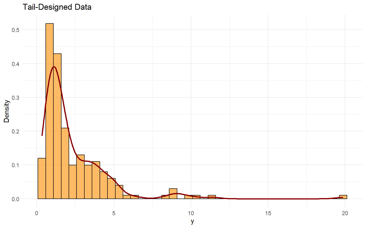
Unconditional CausalMixGPD: Stick-Breaking (SB) Backend with Tail Augmentation

Purpose: Demonstrate the stick-breaking backend (components = J) while augmenting the extreme tail with a GPD. This mirrors the CRP+GPD pipeline (ex03) but highlights the fixed-truncation behavior for bulk components.

What you’ll learn

How to combine SB truncation (components = J) with GPD tail augmentation (GPD = TRUE).
What stays invariant across backends in the wrapper-first workflow: bundle() → dpmgpd() → predict()/plot().
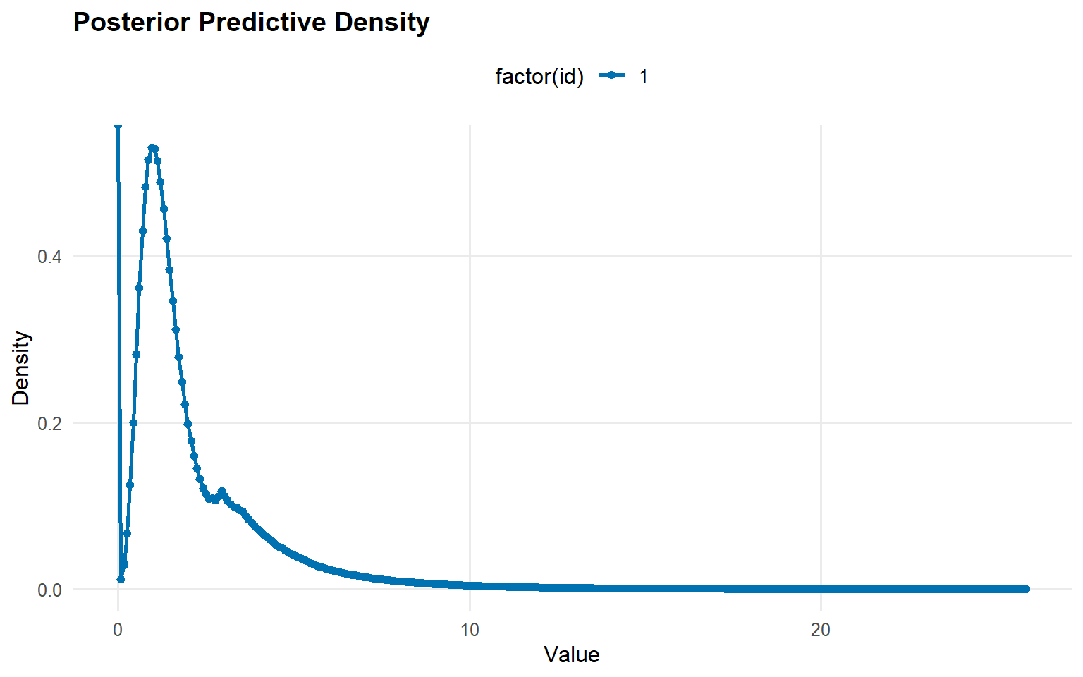
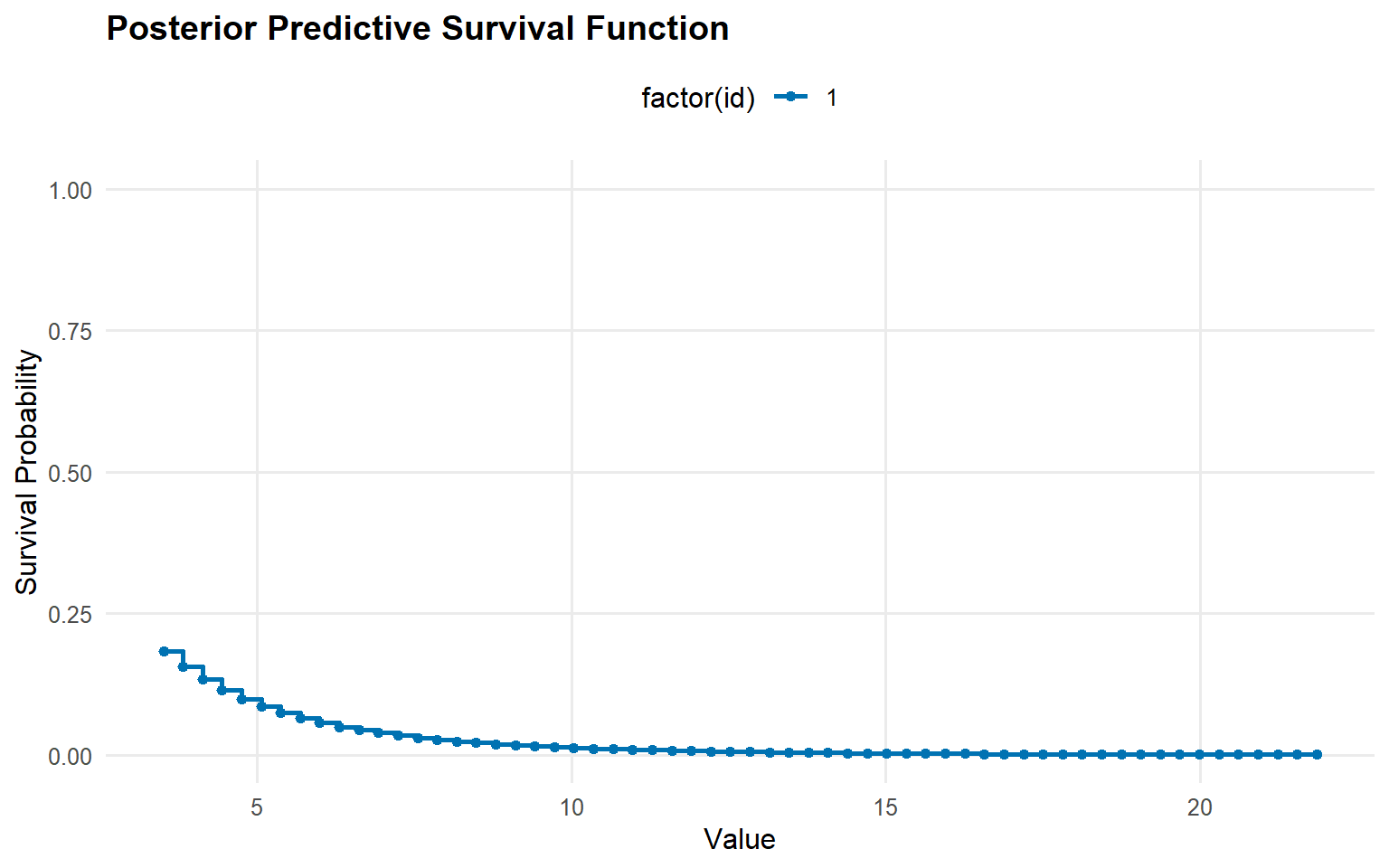
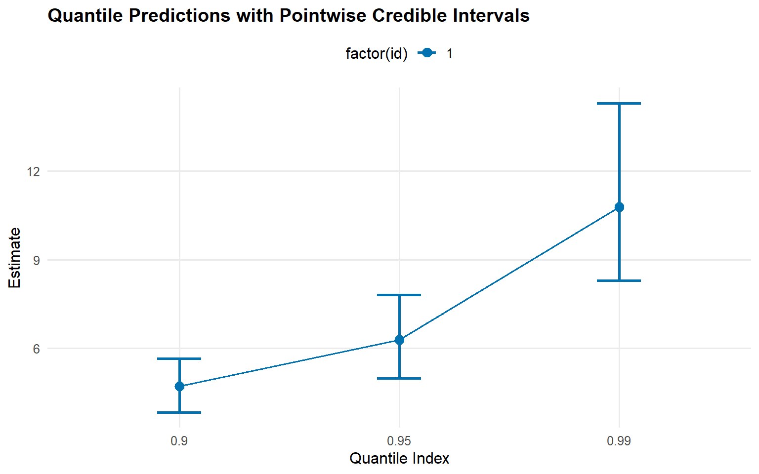
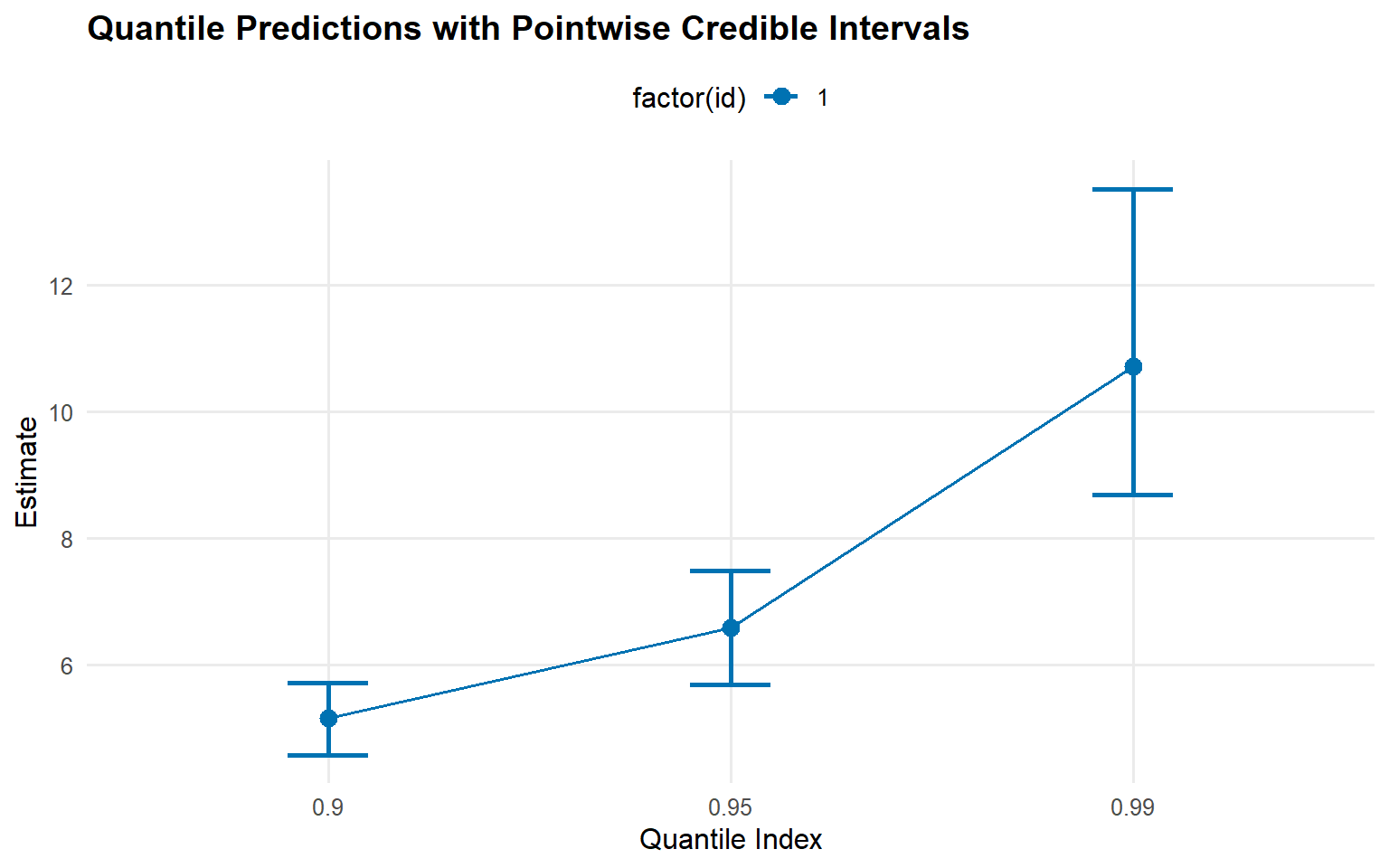
How to sanity-check tail impact using density/survival/high-quantile predictions.

When to use this template

You want tail augmentation and also want the computational predictability of a fixed-component SB mixture.
You want an explicit tuning knob (components) while iterating on model structure.

Next steps

Compare against CRP+GPD (ex03) to see how partition flexibility affects uncertainty.

Data Setup

Code

# Tail-heavy data
data("nc_pos_tail200_k4")
y_tail <- nc_pos_tail200_k4$y

summary_tbl <- tibble(
  statistic = c("N", "Mean", "SD", "Min", "Max"),
  value = c(length(y_tail), mean(y_tail), sd(y_tail), min(y_tail), max(y_tail))
)

df_data <- data.frame(y = y_tail)

p_raw <- ggplot(df_data, aes(x = y)) +
  geom_histogram(aes(y = after_stat(density)), bins = 40, fill = "darkorange", alpha = 0.6, color = "black") +
  geom_density(color = "darkred", linewidth = 1) +
  labs(title = "Tail-Designed Data", x = "y", y = "Density") +
  theme_minimal()

print(p_raw)

# A tibble: 5 × 2
  statistic   value
  <chr>       <dbl>
1 N         200    
2 Mean        2.33 
3 SD          2.30 
4 Min         0.328
5 Max        19.9

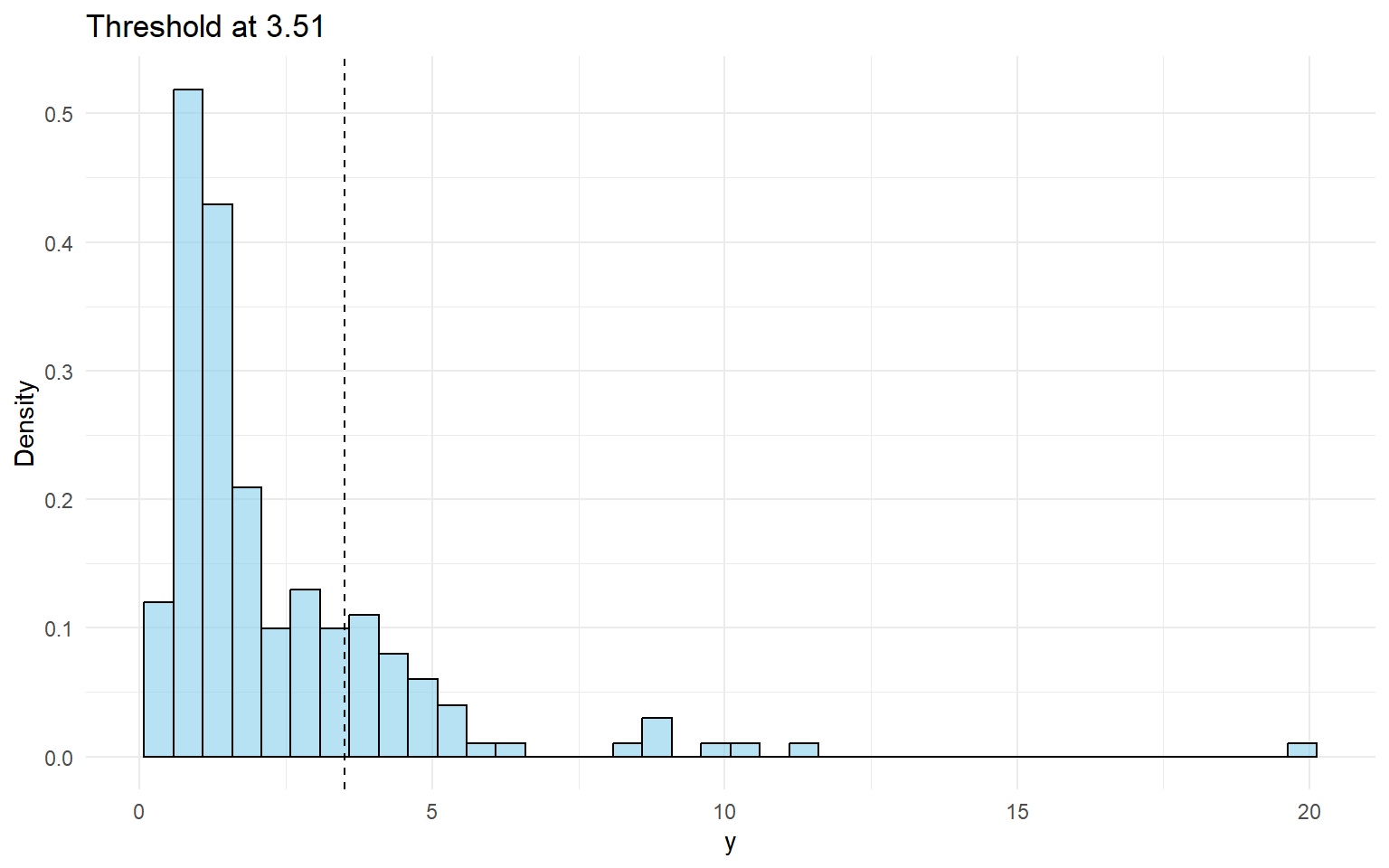
Threshold Selection

Code

thresholds <- quantile(y_tail, c(0.70, 0.75, 0.80, 0.85))
u_threshold <- thresholds["80%"]

ggplot(df_data, aes(x = y)) +
  geom_histogram(aes(y = after_stat(density)), bins = 40, fill = "skyblue", alpha = 0.6, color = "black") +
  geom_vline(xintercept = u_threshold, linetype = "dashed", color = "black") +
  labs(title = paste("Threshold at", round(u_threshold, 2)), x = "y", y = "Density") +
  theme_minimal()

Model Specification & Bundle

This follows the same structure as the SB bulk-only vignette (ex02): build a bundle with bundle(), run MCMC, then use the S3 predict() + plot() helpers. Compared with ex03 (CRP+GPD), here we keep the stick-breaking backend and use a Gamma bulk kernel with a lognormal threshold prior, then contrast it with a bulk-only Laplace fit.

Code

bundle_sb_gpd <- bundle(
  y = y_tail,
  kernel = "gamma",
  backend = "sb",
  GPD = TRUE,
  components = 5,
  param_specs = list(
    gpd = list(
      threshold = list(
        mode = "dist",
        dist = "lognormal",
        args = list(meanlog = log(max(u_threshold, .Machine$double.eps)), sdlog = 0.25)
      )
    )
  ),
  mcmc = mcmc
)

Running MCMC

Code

fit_sb_gpd <- load_or_fit("ex04-unconditional-dpmgpd-sb-fit_sb_gpd", dpmgpd(bundle_sb_gpd))
summary(fit_sb_gpd)

MixGPD summary | backend: Stick-Breaking Process | kernel: Gamma Distribution | GPD tail: TRUE | epsilon: 0.025
n = 200 | components = 5
Summary
Initial components: 5 | Components after truncation: 3

Summary table
  parameter  mean    sd q0.025 q0.500 q0.975    ess
 weights[1] 0.538  0.11  0.346  0.522  0.707   3.37
 weights[2] 0.253 0.063  0.145  0.256  0.351  6.253
 weights[3] 0.139 0.062   0.05  0.126  0.245  3.059
      alpha 1.055 0.417  0.446   1.02  1.971 20.348
 tail_scale 1.981 0.609  1.133  1.833  3.626 12.737
 tail_shape 0.151 0.106 -0.093  0.159  0.349 11.938
  threshold 3.142 0.787   2.39  2.856  5.463  6.018
   shape[1] 4.988 1.095  2.685  4.862  8.108 11.418
   shape[2] 3.051 1.284   1.43  2.744  6.212   9.32
   shape[3]  2.45 1.178  1.108  2.058  5.212  10.48
   scale[1] 0.299 0.204  0.142  0.246  0.993 13.017
   scale[2]  1.86  1.52  0.169  1.323  5.145  3.471
   scale[3]  2.88 1.384  1.175  2.577  6.404 50.099

Code

params_sb_gpd <- params(fit_sb_gpd)
params_sb_gpd

Posterior mean parameters

$alpha
[1] 1.055

$w
[1] 0.5381 0.2532 0.1394

$shape
[1] 4.988 3.051 2.450

$scale
[1] 0.2985 1.8600 2.8800

$tail_scale
[1] 1.981

$tail_shape
[1] 0.1508

Posterior Predictions

Code

y_grid <- seq(0, max(y_tail) * 1.3, length.out = 300)
pred_density <- predict(fit_sb_gpd, y = y_grid, type = "density")
plot(pred_density)

Code

y_surv <- seq(u_threshold, max(y_tail) * 1.1, length.out = 60)
pred_surv <- predict(fit_sb_gpd, y = y_surv, type = "survival")
plot(pred_surv)

Code

quant_probs <- c(0.90, 0.95, 0.99)
pred_quant <- predict(fit_sb_gpd, type = "quantile", p = quant_probs, interval = "credible")
plot(pred_quant)

Tail vs Bulk Comparison

Code

bundle_sb_bulk <- bundle(
  y = y_tail,
  kernel = "laplace",
  backend = "sb",
  GPD = FALSE,
  components = 5,
  mcmc = mcmc
)
fit_sb_bulk <- load_or_fit("ex04-unconditional-dpmgpd-sb-fit_sb_bulk", dpmix(bundle_sb_bulk))

bulk_quant <- predict(fit_sb_bulk, type = "quantile", p = quant_probs)
t_quant <- predict(fit_sb_gpd, type = "quantile", p = quant_probs)

bind_rows(
  bulk_quant$fit %>% mutate(model = "Bulk-only"),
  t_quant$fit %>% mutate(model = "Bulk + GPD")
) %>%
  select(any_of(c("model", "index", "estimate", "lwr", "upr", "lower", "upper")))

       model index  estimate    lower     upper
1  Bulk-only  0.90  5.157292 4.578650  5.722606
2  Bulk-only  0.95  6.583909 5.690428  7.484298
3  Bulk-only  0.99 10.716616 8.691089 13.520645
4 Bulk + GPD  0.90  4.715481 3.840533  5.662347
5 Bulk + GPD  0.95  6.298667 4.983781  7.807621
6 Bulk + GPD  0.99 10.771050 8.290001 14.287834

Code

plot(bulk_quant)

Code

plot(t_quant)

Diagnostics

Code

plot(fit_sb_gpd, family = c("histogram", "autocorrelation", "running"))


=== histogram ===


=== autocorrelation ===


=== running ===

Key Takeaways

Stick-breaking truncation fixes the number of bulk components but still flexibly models the tail via GPD.
Posterior predict() + plot() workflows visualize densities, survival probabilities, and posterior-mean extreme quantiles.
Comparing bulk-only vs GPD-augmented quantiles reveals how tail augmentation shifts the 95-99% levels.
Next: conditional DPM (ex05-ex08) to explore covariate effects before moving to causal regimes.

Prereqs

Required packages and data for this page are listed in the setup chunks above.

Outputs

This page renders model fits, diagnostics, and summary artifacts generated by package APIs.

Interpretation

Canonical concept page: Model Umbrella
Treat this page as an application/example view and use the canonical page for core definitions.

Continue to the linked canonical concept page, then return for implementation-specific details.

Unconditional CausalMixGPD: Stick-Breaking (SB) Backend with Tail Augmentation

What you’ll learn

When to use this template

Next steps

Data Setup

Threshold Selection

Model Specification & Bundle

Running MCMC

Posterior Predictions

Tail vs Bulk Comparison

Diagnostics

Key Takeaways

Workflow Navigation

Prereqs

Outputs

Interpretation

Next