Website workflow note. This page reflects the current exported API and recommended wrapper-first usage. Last updated: 2026-02-19.
For the full package narrative, see the main package vignettes (basic, unconditional, conditional, and causal).
Conditional DPmix: CRP Backend with Covariates
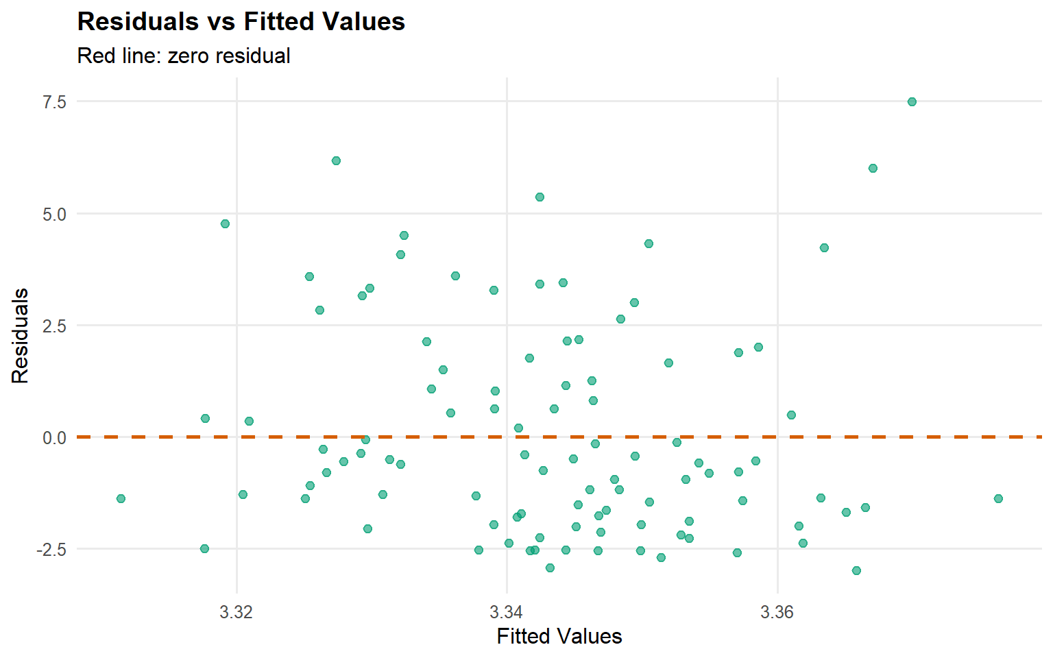
Purpose: Show how the CRP backend can model \(y | X\) via a covariate-dependent Dirichlet Process mixture. This vignette parallels start/backends-and-workflow but includes \(X\) so we can explore conditional predictions.
What you’ll learn
How to fit a conditional DP mixture (y \mid X) with the CRP backend.
How to form covariate-slice predictions with predict(fit, newdata = X_new, ...) and interpret them.
How kernel choice affects conditional fit even when GPD = FALSE.
When to use this template
You want flexible conditional density estimation (p(y \mid X)) without committing to a parametric regression form.
You expect heteroskedasticity, skewness, or multimodality that can vary with (X).
Next steps
If extremes matter for some covariate regions, extend to conditional tail modeling (ex07/ex08).
Data Setup
Code
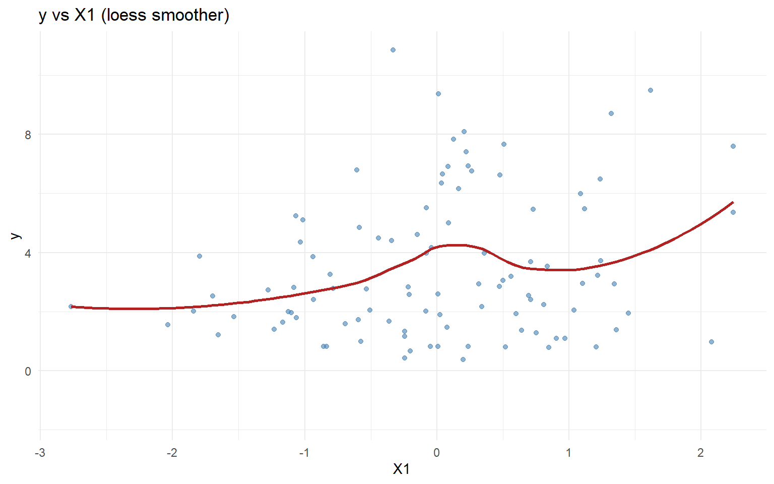
data("nc_posX100_p3_k2")y <- nc_posX100_p3_k2$yX <-as.matrix(nc_posX100_p3_k2$X)if (is.null(colnames(X))) {colnames(X) <-paste0("x", seq_len(ncol(X)))}summary_tbl <-tibble(statistic =c("N", "Mean", "SD", "Min", "Max"),value =c(length(y), mean(y), sd(y), min(y), max(y)))df_cov <-data.frame(y = y, x1 = X[, 1], x2 = X[, 2])p_cov <-ggplot(df_cov, aes(x = x1, y = y)) +geom_point(alpha =0.6, color ="steelblue") +geom_smooth(method ="loess", color ="firebrick", fill =NA) +labs(title ="y vs X1 (loess smoother)", x ="X1", y ="y") +theme_minimal()print(p_cov)
Code
summary_tbl
# A tibble: 5 × 2
  statistic   value
  <chr>       <dbl>
1 N         100
2 Mean        3.45
3 SD          2.41
4 Min         0.377
5 Max        10.9