ex06. Conditional DPM (SB Backend)

Website workflow note. This page reflects the current exported API and recommended wrapper-first usage. Last updated: 2026-02-19.

For the full package narrative, see the main package vignettes (basic, unconditional, conditional, and causal).

Conditional DPmix: Stick-Breaking Backend

Purpose: Replace the CRP backend with stick-breaking truncation while keeping the covariate-dependent bulk structure. This demonstrates how fixed components interplay with covariates.

What you’ll learn

How to run the conditional (y \mid X) workflow using the SB backend (fixed truncation).
How components controls effective mixture complexity in conditional fits.
How to compare kernels under the same SB setup using parallel bundles.

When to use this template

You want conditional density estimation with predictable runtime and a tunable complexity knob (components).
You want conditional modeling but do not need tail splicing (GPD = FALSE).

Next steps

Add tail augmentation for covariate-dependent extremes (ex08), or compare with CRP conditional (ex05).

Data Setup

Code

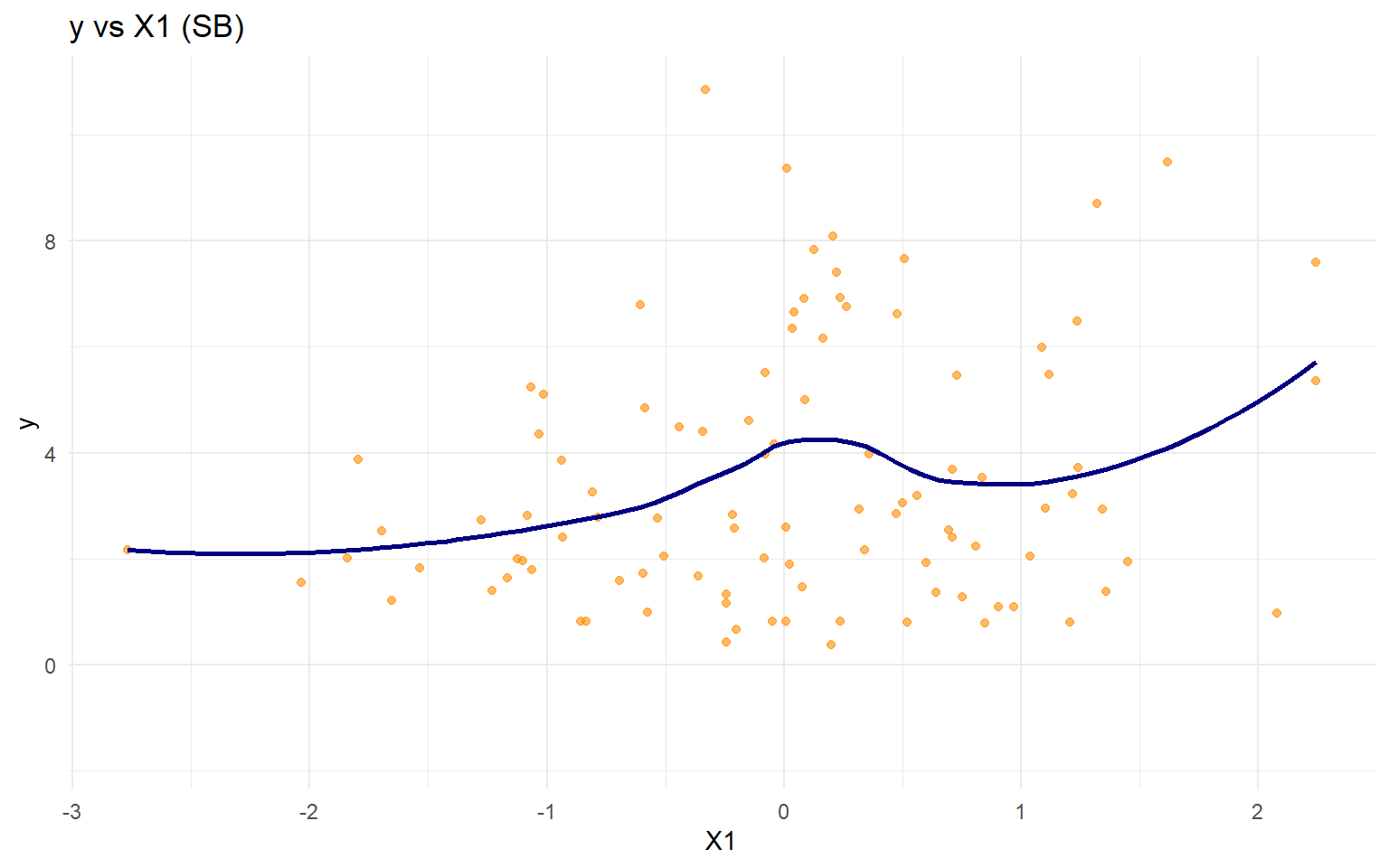
data("nc_posX100_p3_k2")
y <- nc_posX100_p3_k2$y
X <- as.matrix(nc_posX100_p3_k2$X)
if (is.null(colnames(X))) {
  colnames(X) <- paste0("x", seq_len(ncol(X)))
}

summary_tbl <- tibble(
  statistic = c("N", "Mean", "SD", "Min", "Max"),
  value = c(length(y), mean(y), sd(y), min(y), max(y))
)

ggplot(data.frame(y = y, x1 = X[, 1]), aes(x = x1, y = y)) +
  geom_point(alpha = 0.6, color = "darkorange") +
  geom_smooth(method = "loess", color = "navy", fill = NA) +
  labs(title = "y vs X1 (SB)", x = "X1", y = "y") +
  theme_minimal()

# A tibble: 5 × 2
  statistic   value
  <chr>       <dbl>
1 N         100    
2 Mean        3.45 
3 SD          2.41 
4 Min         0.377
5 Max        10.9

Model Specification

Code

bundle_sb_normal <- bundle(
  y = y,
  X = X,
  kernel = "normal",
  backend = "sb",
  GPD = FALSE,
  components = 5,
  mcmc = mcmc
)

bundle_sb_cauchy <- bundle(
  y = y,
  X = X,
  kernel = "cauchy",
  backend = "sb",
  GPD = FALSE,
  components = 5,
  mcmc = mcmc
)

Running MCMC

Code

fit_sb_normal <- load_or_fit("ex06-conditional-dpm-sb-fit_sb_normal", dpmix(bundle_sb_normal))
fit_sb_cauchy <- load_or_fit("ex06-conditional-dpm-sb-fit_sb_cauchy", dpmix(bundle_sb_cauchy))
summary(fit_sb_normal)

MixGPD summary | backend: Stick-Breaking Process | kernel: Normal Distribution | GPD tail: FALSE | epsilon: 0.025
n = 100 | components = 5
Summary
Initial components: 5 | Components after truncation: 2

Summary table
       parameter   mean    sd q0.025 q0.500 q0.975    ess
      weights[1]   0.71 0.125  0.432  0.717  0.891  2.821
      weights[2]  0.188 0.091  0.075  0.139  0.353  3.134
           alpha  0.973 0.467  0.266  0.836  2.086 30.527
 beta_mean[1, 1] -0.697 0.689 -2.269 -0.399  0.193  3.626
 beta_mean[2, 1]  0.874 0.527 -0.155  1.016  1.891  3.601
 beta_mean[3, 1]  -0.21 0.482 -1.133 -0.228  0.599 11.882
 beta_mean[4, 1]  -0.86 0.553 -1.798 -0.897  0.353   6.33
 beta_mean[5, 1]  0.552 0.522 -1.185  0.581  1.235  8.768
 beta_mean[1, 2]  1.274 0.846  0.465  0.976  3.069  2.147
 beta_mean[2, 2]    0.3  0.45 -0.736  0.399  1.115  8.059
 beta_mean[3, 2] -0.982 0.425  -1.82 -0.838 -0.251 12.352
 beta_mean[4, 2]  -0.33 0.314 -1.136 -0.367  0.335 29.796
 beta_mean[5, 2]  2.136 0.702  1.518  1.919  3.718  2.955
 beta_mean[1, 3] -0.464 0.897 -2.007 -0.273  0.447  2.248
 beta_mean[2, 3]  0.336 0.852 -0.594  0.263  1.843  1.602
 beta_mean[3, 3] -1.703 0.564 -2.487 -1.858 -0.072  6.078
 beta_mean[4, 3]  0.792 0.817 -0.046  0.432  2.963  2.573
 beta_mean[5, 3]  1.737 0.812  0.548  1.701  3.785  3.443
           sd[1]  0.053  0.01  0.036  0.053  0.073 52.239
           sd[2]  0.794 1.107  0.037  0.234  3.846 22.413

Code

summary(fit_sb_cauchy)

MixGPD summary | backend: Stick-Breaking Process | kernel: Cauchy Distribution | GPD tail: FALSE | epsilon: 0.025
n = 100 | components = 5
Summary
Initial components: 5 | Components after truncation: 3

Summary table
           parameter   mean    sd q0.025 q0.500 q0.975     ess
          weights[1]  0.435 0.078  0.297  0.447  0.573   8.109
          weights[2]  0.285 0.049  0.189    0.3   0.35  10.355
          weights[3]   0.17 0.046  0.083  0.172  0.258   11.74
               alpha  1.381 0.846  0.319  1.133  3.513  17.696
 beta_location[1, 1]  1.031 1.408 -1.795  1.507  2.522   1.503
 beta_location[2, 1]  1.135 0.786 -0.182  1.183   2.12   4.936
 beta_location[3, 1]  0.758 1.099 -1.514  0.772  2.525   3.277
 beta_location[4, 1]  0.153 0.777 -0.631 -0.184  1.832   2.518
 beta_location[5, 1]  0.091 0.661 -0.979  0.309  1.353   9.197
 beta_location[1, 2]  0.532 0.927 -0.891  0.133  2.046    2.91
 beta_location[2, 2] -1.785 1.241 -3.511  -1.88  0.311    2.29
 beta_location[3, 2] -3.126 1.533 -4.652 -3.934  0.302   1.866
 beta_location[4, 2] -1.304 1.338 -3.017 -1.371  1.447   2.479
 beta_location[5, 2]  1.507 0.419  0.527  1.623   2.03   9.906
 beta_location[1, 3]  1.058 0.827 -1.123   0.94  2.358    4.52
 beta_location[2, 3]  1.654 1.804 -2.067   2.43  3.752   2.449
 beta_location[3, 3]  1.364 1.264 -1.047  1.404  2.961   2.195
 beta_location[4, 3]  -1.01 1.051 -2.325  -1.35  1.259   1.961
 beta_location[5, 3]  -1.34 1.028 -3.261 -1.114    0.3   2.243
            scale[1]  2.046  0.56   1.16  1.964  3.233 103.998
            scale[2]   2.19  0.82  0.978  2.027  4.075  78.988
            scale[3]   1.99 0.966  0.612  1.788  4.133  82.816

Code

params_sb <- params(fit_sb_normal)
params_sb

Posterior mean parameters

$alpha
[1] 0.9726

$w
[1] 0.7103 0.1881

$beta_mean
           x1      x2      x3
comp1 -0.6969  1.2740 -0.4642
comp2  0.8744  0.3004  0.3364
comp3 -0.2103 -0.9816 -1.7030
comp4 -0.8597 -0.3299  0.7915
comp5  0.5520  2.1360  1.7370

$sd
[1] 0.05346 0.79370

Conditional Predictive Density

Code

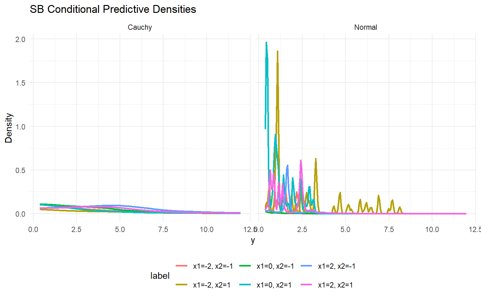
X_new <- expand.grid(x1 = seq(-2, 2, length.out = 3), x2 = c(-1, 1), x3 = 0)
colnames(X_new) <- colnames(X)
y_min <- max(min(y), .Machine$double.eps)
y_grid <- seq(y_min, max(y) * 1.1, length.out = 200)

densities_normal <- lapply(seq_len(nrow(X_new)), function(i) {
  pred <- predict(fit_sb_normal, newdata =as.matrix(X_new[i, , drop = FALSE]), y = y_grid, type = "density")
  data.frame(
    y = pred$fit$y,
    density = pred$fit$density,
    label = paste0("x1=", round(X_new[i, "x1"], 1), ", x2=", X_new[i, "x2"]),
    model = "Normal"
  )
})

densities_cauchy <- lapply(seq_len(nrow(X_new)), function(i) {
  pred <- predict(fit_sb_cauchy, newdata =as.matrix(X_new[i, , drop = FALSE]), y = y_grid, type = "density")
  data.frame(
    y = pred$fit$y,
    density = pred$fit$density,
    label = paste0("x1=", round(X_new[i, "x1"], 1), ", x2=", X_new[i, "x2"]),
    model = "Cauchy"
  )
})

df_cond <- bind_rows(densities_normal, densities_cauchy)

ggplot(df_cond, aes(x = y, y = density, color = label)) +
  geom_line(linewidth = 1) +
  facet_wrap(~ model) +
  labs(title = "SB Conditional Predictive Densities", x = "y", y = "Density") +
  theme_minimal() +
  theme(legend.position = "bottom")

Quantile Drift with Covariates

Code

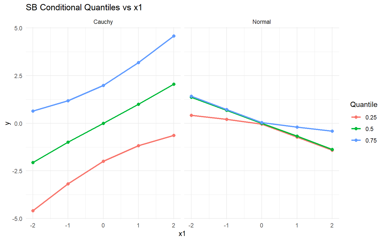
X_eval <- cbind(x1 = seq(-2, 2, length.out = 5), x2 = 0, x3 = 0)
colnames(X_eval) <- colnames(X)
quant_probs <- c(0.25, 0.5, 0.75)

pred_q_normal <- predict(fit_sb_normal, newdata =as.matrix(X_eval), type = "quantile", p = quant_probs)
pred_q_cauchy <- predict(fit_sb_cauchy, newdata =as.matrix(X_eval), type = "quantile", p = quant_probs)

quant_df_normal <- pred_q_normal$fit
quant_df_normal$x1 <- X_eval[quant_df_normal$id, "x1"]
quant_df_normal$model <- "Normal"

quant_df_cauchy <- pred_q_cauchy$fit
quant_df_cauchy$x1 <- X_eval[quant_df_cauchy$id, "x1"]
quant_df_cauchy$model <- "Cauchy"

bind_rows(quant_df_normal, quant_df_cauchy) %>%
  ggplot(aes(x = x1, y = estimate, color = factor(index), group = index)) +
  geom_line(linewidth = 1) +
  geom_point(size = 2) +
  facet_wrap(~ model) +
  labs(title = "SB Conditional Quantiles vs x1", x = "x1", y = "y", color = "Quantile") +
  theme_minimal()

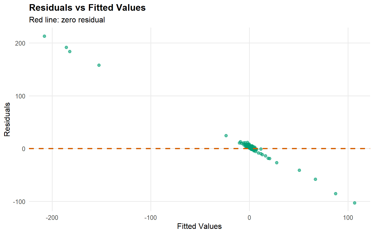
Residuals & Diagnostics

Code

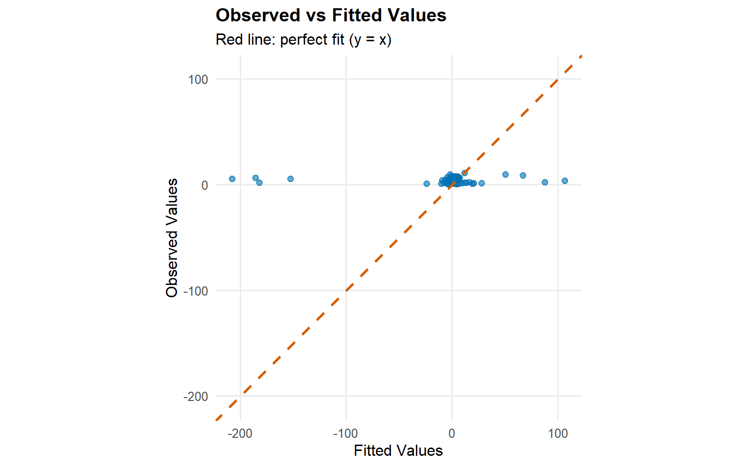
plot(fitted(fit_sb_cauchy))

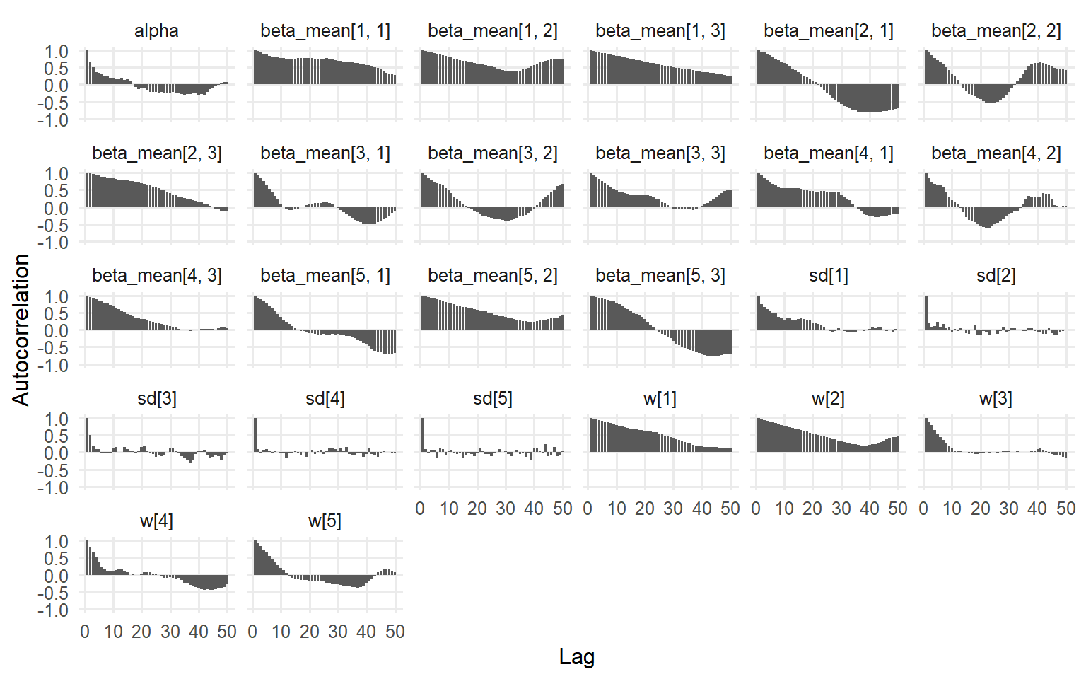
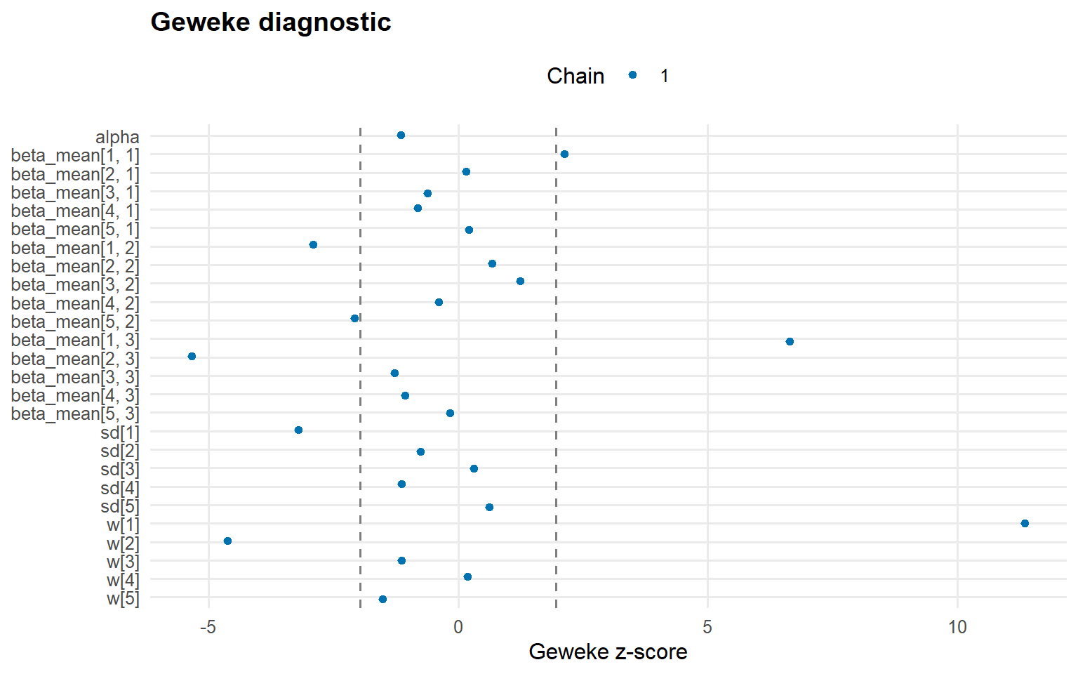
Code

plot(fit_sb_normal, family = c("traceplot", "autocorrelation", "geweke"))


=== traceplot ===


=== autocorrelation ===


=== geweke ===

Code

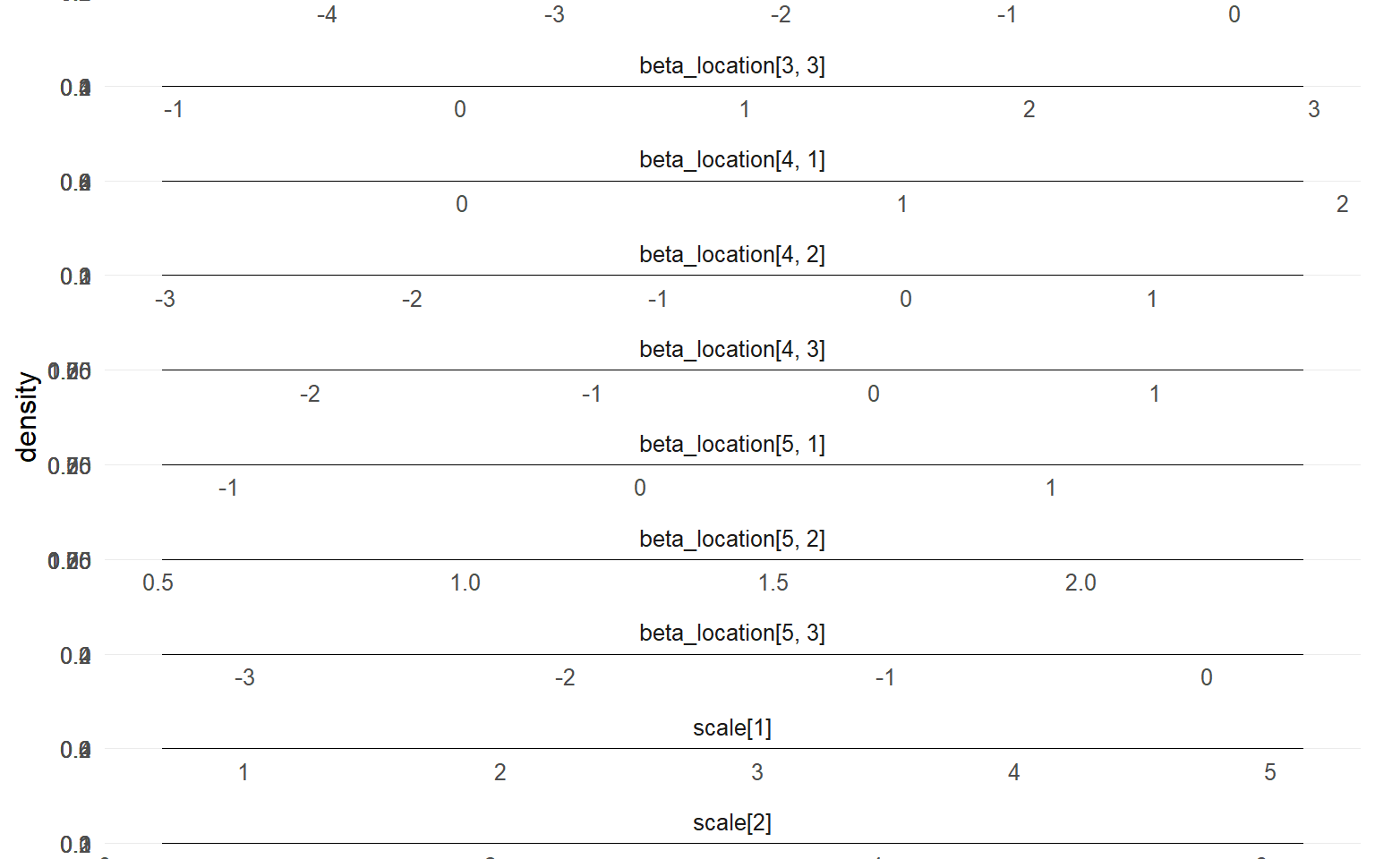
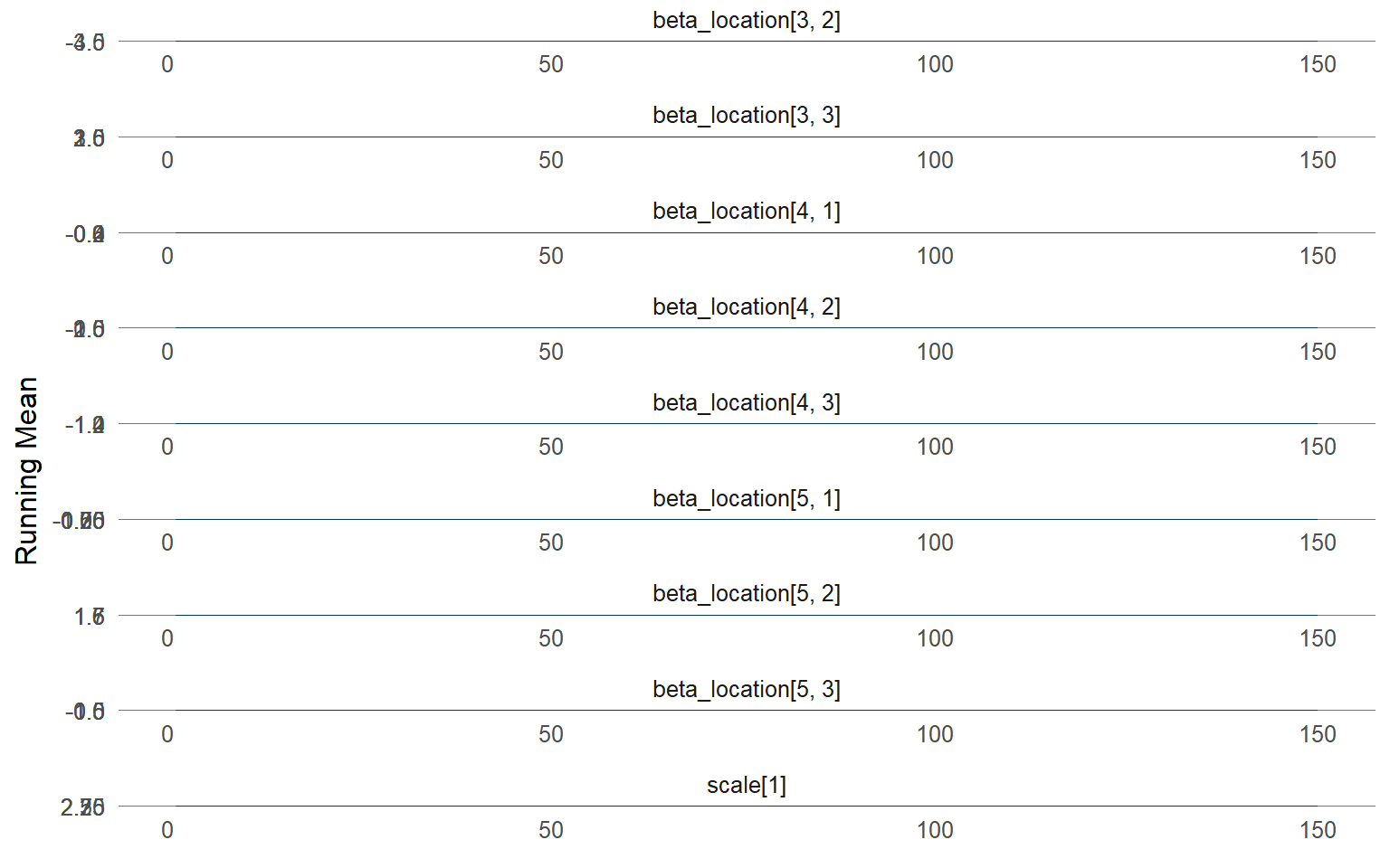
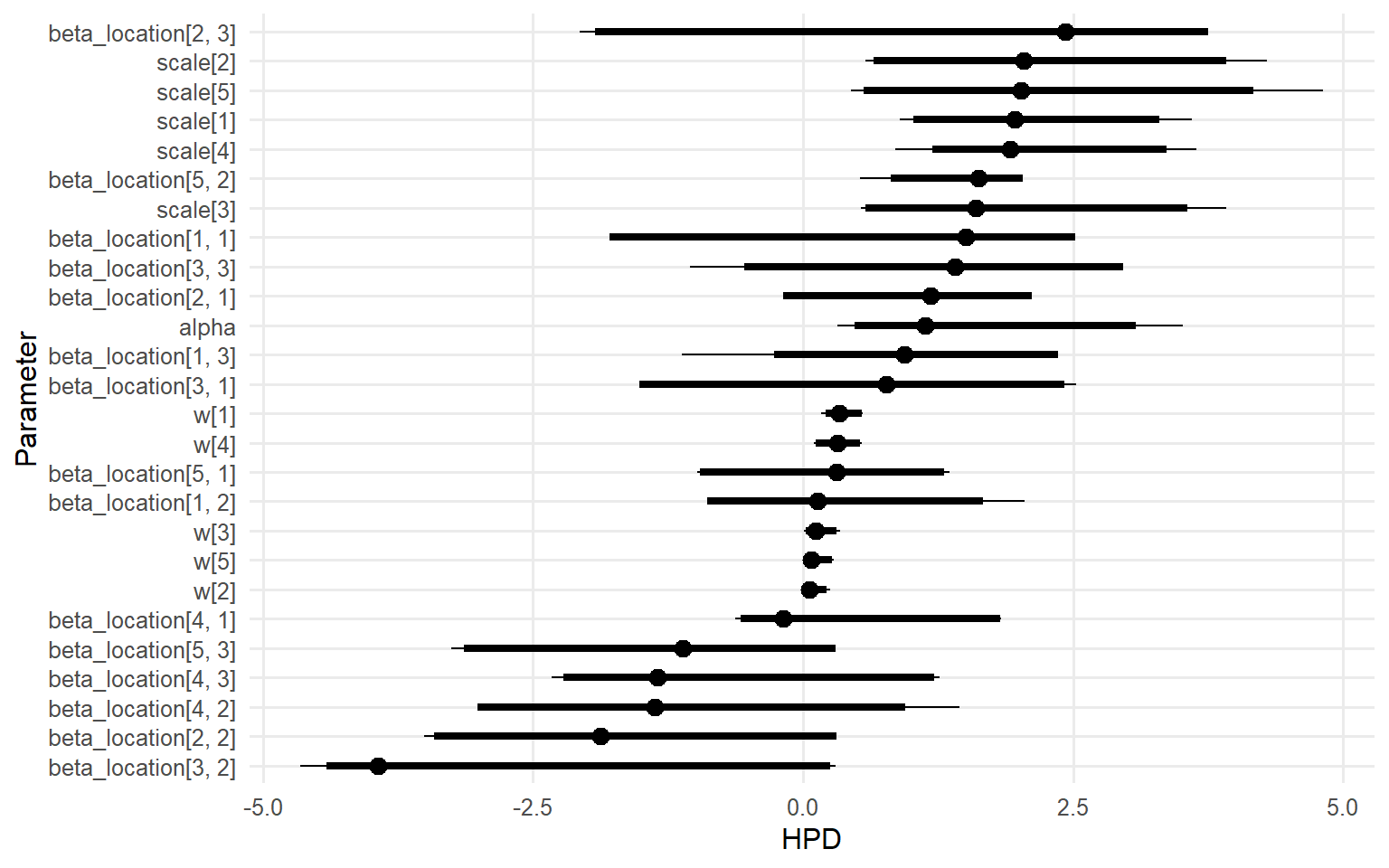
plot(fit_sb_cauchy, family = c("density", "running", "caterpillar"))


=== density ===


=== running ===


=== caterpillar ===

Takeaways

Stick-breaking component count is fixed but still supports covariate-dependent mixtures.
predict(..., type = "density") returns group-specific densities for each X.
predict(..., type = "quantile") reports posterior-mean quantiles; the median is the 0.5 quantile and shifts with x1.
Diagnoses rely on the same S3 plot()/fitted() pipeline available in other vignettes.

Prereqs

Required packages and data for this page are listed in the setup chunks above.

Outputs

This page renders model fits, diagnostics, and summary artifacts generated by package APIs.

Interpretation

Canonical concept page: Model Umbrella
Treat this page as an application/example view and use the canonical page for core definitions.

Continue to the linked canonical concept page, then return for implementation-specific details.

Conditional DPmix: Stick-Breaking Backend

What you’ll learn

When to use this template

Next steps

Data Setup

Model Specification

Running MCMC

Conditional Predictive Density

Quantile Drift with Covariates

Residuals & Diagnostics

Takeaways

Workflow Navigation

Prereqs

Outputs

Interpretation

Next