ex07. Conditional DPMGPD (CRP Backend)

Website workflow note. This page reflects the current exported API and recommended wrapper-first usage. Last updated: 2026-02-19.

For the full package narrative, see the main package vignettes (basic, unconditional, conditional, and causal).

Conditional CausalMixGPD: CRP Backend with Tail Augmentation

Purpose: Combine conditional modeling with GPD tail augmentation so each covariate slice inherits both mixture bulk and tail behavior. This extends the unconditional GPD (ex03) and conditional DP (ex05).

What you’ll learn

How to model (y X) when both the bulk shape and the extreme tail matter.
How conditional tail modeling changes what you can query from predict() (survival/high quantiles per covariate slice).
How to encode threshold behavior via param_specs in a conditional setting.

When to use this template

Extremes matter and may depend on (X) (risk modeling, rare-event probability statements).
You want a flexible bulk model but do not want tail behavior to be implicitly driven by the bulk kernel alone.

Next steps

Swap CRP for SB (ex08) to compare truncation vs partition flexibility under the same tail-augmented goal.

Data Setup

Code

data("nc_posX100_p5_k4")
y <- nc_posX100_p5_k4$y
X <- as.matrix(nc_posX100_p5_k4$X)
if (is.null(colnames(X))) {
  colnames(X) <- paste0("x", seq_len(ncol(X)))
}

summary_tbl <- tibble(
  statistic = c("N", "Mean", "SD", "Min", "Max"),
  value = c(length(y), mean(y), sd(y), min(y), max(y))
)

ggplot(data.frame(y = y, x1 = X[, 1]), aes(x = x1, y = y)) +
  geom_point(alpha = 0.5, color = "darkgreen") +
  geom_smooth(method = "loess", color = "steelblue", fill = NA) +
  labs(title = "Outcome vs X1 (Tail dataset)", x = "X1", y = "y") +
  theme_minimal()

Code

summary_tbl

# A tibble: 5 × 2
  statistic   value
  <chr>       <dbl>
1 N         100    
2 Mean        1.94 
3 SD          1.15 
4 Min         0.488
5 Max         5.28

Threshold Selection

Code

u_threshold <- quantile(y, 0.85)

ggplot(data.frame(y = y), aes(x = y)) +
  geom_histogram(aes(y = after_stat(density)), bins = 40, fill = "magenta", alpha = 0.6, color = "black") +
  geom_vline(xintercept = u_threshold, linetype = "dashed", color = "black") +
  labs(title = paste("Threshold at", signif(u_threshold, 3)), x = "y", y = "Density") +
  theme_minimal()

Model Specification & Bundle

Code

bundle_cond_gpd_lognormal <- bundle(
  y = y,
  X = X,
  kernel = "lognormal",
  backend = "crp",
  GPD = TRUE,
  components = 5,
  param_specs = list(
    gpd = list(
      threshold = list(mode = "link", link = "exp")
    )
  ),
  mcmc = mcmc
)

bundle_cond_gpd_normal <- bundle(
  y = y,
  X = X,
  kernel = "normal",
  backend = "crp",
  GPD = TRUE,
  components = 5,
  param_specs = list(
    gpd = list(
      threshold = list(mode = "link", link = "exp")
    )
  ),
  mcmc = mcmc
)

Running MCMC

Code

fit_cond_gpd_lognormal <- load_or_fit("ex07-conditional-dpmgpd-crp-fit_cond_gpd_lognormal", dpmgpd(bundle_cond_gpd_lognormal))
fit_cond_gpd_normal <- load_or_fit("ex07-conditional-dpmgpd-crp-fit_cond_gpd_normal", dpmgpd(bundle_cond_gpd_normal))
summary(fit_cond_gpd_lognormal)

MixGPD summary | backend: Chinese Restaurant Process | kernel: Lognormal Distribution | GPD tail: TRUE | epsilon: 0.025
n = 100 | components = 5
Summary
Initial components: 5 | Components after truncation: 1

WAIC: 284.282
lppd: -137.272 | pWAIC: 4.869

Summary table
          parameter   mean    sd q0.025 q0.500 q0.975     ess
         weights[1]  0.988 0.036   0.85      1      1  15.629
              alpha  0.256 0.236  0.003   0.18  0.827     150
 beta_tail_scale[1]  0.218 0.117  0.004  0.224  0.446 193.979
 beta_tail_scale[2]      0 0.194  -0.36  0.015  0.371     150
 beta_tail_scale[3] -0.014 0.099 -0.203 -0.019  0.186 173.001
 beta_tail_scale[4]  0.501 0.246  0.051  0.504  0.991     150
 beta_tail_scale[5]  -0.06 0.109 -0.279 -0.067  0.152     150
  beta_threshold[1]      0     0      0      0      0       0
  beta_threshold[2]      0     0      0      0      0       0
  beta_threshold[3]      0     0      0      0      0       0
  beta_threshold[4]      0     0      0      0      0       0
  beta_threshold[5]      0     0      0      0      0       0
         tail_shape -0.012 0.099 -0.165 -0.004  0.183  32.624
         meanlog[1]  0.311 0.081  0.196  0.293  0.497  17.976
           sdlog[1]  0.474  0.07  0.362  0.469  0.634  30.183

Code

summary(fit_cond_gpd_normal)

MixGPD summary | backend: Chinese Restaurant Process | kernel: Normal Distribution | GPD tail: TRUE | epsilon: 0.025
n = 100 | components = 5
Summary
Initial components: 5 | Components after truncation: 1

WAIC: 286.63
lppd: -138.407 | pWAIC: 4.908

Summary table
          parameter   mean    sd q0.025 q0.500 q0.975     ess
         weights[1]  0.989 0.036   0.86      1      1  18.416
              alpha  0.194 0.203   0.01  0.124  0.769   50.53
 beta_tail_scale[1]  0.223 0.111 -0.005  0.222  0.434     150
 beta_tail_scale[2]  0.011 0.179  -0.36 -0.003   0.34 107.097
 beta_tail_scale[3] -0.016 0.095 -0.196 -0.021  0.163 283.425
 beta_tail_scale[4]  0.566 0.235  0.111  0.543  0.996  73.362
 beta_tail_scale[5] -0.051 0.103 -0.248 -0.057  0.142  94.408
  beta_threshold[1]      0     0      0      0      0       0
  beta_threshold[2]      0     0      0      0      0       0
  beta_threshold[3]      0     0      0      0      0       0
  beta_threshold[4]      0     0      0      0      0       0
  beta_threshold[5]      0     0      0      0      0       0
         tail_shape -0.065 0.102 -0.274 -0.068  0.156  20.198
            mean[1]  1.248 0.068  1.144  1.261   1.36   7.203
              sd[1]  0.398 0.077  0.271   0.39  0.546   5.942

Code

params_cond_gpd <- params(fit_cond_gpd_lognormal)
params_cond_gpd

Posterior mean parameters

$alpha
[1] 0.256

$w
[1] 0.9878

$meanlog
[1] 0.3111

$sdlog
[1] 0.4738

$beta_threshold
[1] 0 0 0 0 0

$beta_tail_scale
[1]  0.2178000  0.0004566 -0.0143500  0.5012000 -0.0596100

$tail_shape
[1] -0.01164

Conditional Tail-aware Predictions

Code

X_new <- rbind(
  c(-1, 0, 0, 0, 0),
  c(0, 0, 0, 0, 0),
  c(1, 1, 0, 0, 0)
)
colnames(X_new) <- colnames(X)
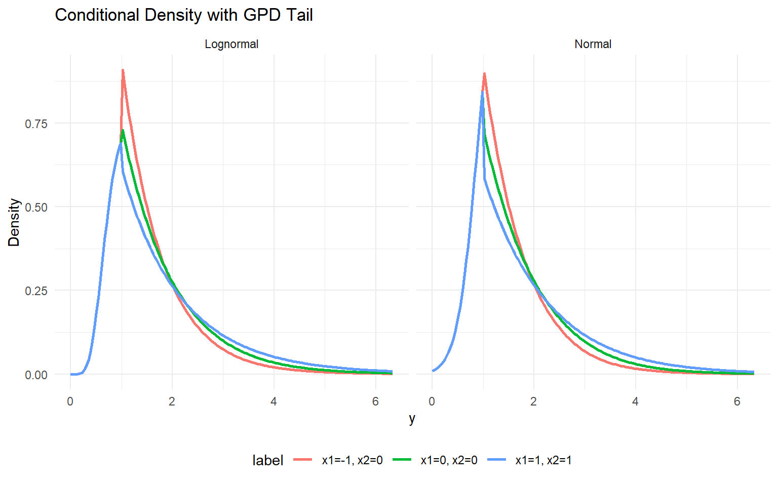
y_grid <- seq(0, max(y) * 1.2, length.out = 200)

df_pred_lognormal <- lapply(seq_len(nrow(X_new)), function(i) {
  pred <- predict(fit_cond_gpd_lognormal, newdata =as.matrix(X_new[i, , drop = FALSE]), y = y_grid, type = "density")
  data.frame(
    y = pred$fit$y,
    density = pred$fit$density,
    label = paste("x1=", X_new[i, 1], ", x2=", X_new[i, 2], sep = ""),
    model = "Lognormal"
  )
})

df_pred_normal <- lapply(seq_len(nrow(X_new)), function(i) {
  pred <- predict(fit_cond_gpd_normal, newdata =as.matrix(X_new[i, , drop = FALSE]), y = y_grid, type = "density")
  data.frame(
    y = pred$fit$y,
    density = pred$fit$density,
    label = paste("x1=", X_new[i, 1], ", x2=", X_new[i, 2], sep = ""),
    model = "Normal"
  )
})

bind_rows(df_pred_lognormal, df_pred_normal) %>%
  ggplot(aes(x = y, y = density, color = label)) +
  geom_line(linewidth = 1) +
  facet_wrap(~ model) +
  labs(title = "Conditional Density with GPD Tail", x = "y", y = "Density") +
  theme_minimal() +
  theme(legend.position = "bottom")

Tail Quantiles vs Covariates

Code

X_grid <- cbind(x1 = seq(-1, 1, length.out = 5), x2 = 0, x3 = 0, x4 = 0, x5 = 0)
colnames(X_grid) <- colnames(X)
quant_probs <- c(0.90, 0.95)

pred_q_lognormal <- predict(fit_cond_gpd_lognormal, newdata =as.matrix(X_grid), type = "quantile", p = quant_probs)
pred_q_normal <- predict(fit_cond_gpd_normal, newdata =as.matrix(X_grid), type = "quantile", p = quant_probs)

quant_df_lognormal <- pred_q_lognormal$fit
quant_df_lognormal$x1 <- X_grid[quant_df_lognormal$id, "x1"]
quant_df_lognormal$model <- "Lognormal"

quant_df_normal <- pred_q_normal$fit
quant_df_normal$x1 <- X_grid[quant_df_normal$id, "x1"]
quant_df_normal$model <- "Normal"

bind_rows(quant_df_lognormal, quant_df_normal) %>%
  ggplot(aes(x = x1, y = estimate, color = factor(index), group = index)) +
  geom_line(linewidth = 1) +
  geom_point(size = 2) +
  facet_wrap(~ model) +
  labs(title = "Tail Quantiles vs x1 (CRP)", x = "x1", y = "Quantile", color = "Probability") +
  theme_minimal()

Residuals & Diagnostics

Code

plot(fitted(fit_cond_gpd_lognormal))

Code

plot(fit_cond_gpd_lognormal, family = c("traceplot", "density", "autocorrelation"))


=== traceplot ===


=== density ===


=== autocorrelation ===

Code

plot(fit_cond_gpd_normal, family = c("running", "geweke", "caterpillar"))


=== running ===


=== geweke ===


=== caterpillar ===

Takeaways

Conditional DPmix with a GPD tail lets posterior-mean extreme quantiles vary with covariates.
The CRP backend samples the bulk and tail jointly while thresholding at the 85th percentile.
predict() + plot() remain the main tools for densities, survival curves, and quantiles; residual diagnostics check fit quality.
Next: Mirror this workflow with the SB backend in ex08.

Prereqs

Required packages and data for this page are listed in the setup chunks above.

Outputs

This page renders model fits, diagnostics, and summary artifacts generated by package APIs.

Interpretation

Canonical concept page: Model Umbrella
Treat this page as an application/example view and use the canonical page for core definitions.

Continue to the linked canonical concept page, then return for implementation-specific details.

Conditional CausalMixGPD: CRP Backend with Tail Augmentation

What you’ll learn

When to use this template

Next steps

Data Setup

Threshold Selection

Model Specification & Bundle

Running MCMC

Conditional Tail-aware Predictions

Tail Quantiles vs Covariates

Residuals & Diagnostics

Takeaways

Workflow Navigation

Prereqs

Outputs

Interpretation

Next