ex10. Causal (X, no PS, SB Backend) - InvGauss/Amoroso

Website workflow note. This page reflects the current exported API and recommended wrapper-first usage. Last updated: 2026-02-19.

For the full package narrative, see the main package vignettes (basic, unconditional, conditional, and causal).

Causal Inference: X Without PS (CRP+SB)

What you’ll learn

How to run the causal workflow with outcome models conditional on X while disabling propensity-score estimation.
How to compare causal fits that differ in backend/tail specification while keeping the same evaluation pattern.
How tail augmentation can change effect behavior in extremes even when mean effects are similar.

When to use this template

Treatment assignment is plausibly ignorable given (X), but you want to avoid PS modeling (or you already handled PS externally).
You want causal summaries beyond the mean (quantile/conditional effects) and need flexible outcome distributions.

Key limitation (important)

With PS disabled, you rely entirely on the outcome models for adjustment. If overlap/positivity is weak, effects can be unstable; use diagnostic plots and sensitivity checks.

What this page does

This vignette uses covariates X but disables PS estimation. Outcome models are conditional on X only.

Model A: CRP with GPD tail (InvGauss)
Model B: SB bulk-only (Amoroso)

Data Setup

Code

data("causal_alt_real500_p4_k2")
y <- abs(causal_alt_real500_p4_k2$y) + 0.01
A <- causal_alt_real500_p4_k2$A
X <- as.matrix(causal_alt_real500_p4_k2$X)

summary_tbl <- tibble(
  statistic = c("N", "Mean", "SD", "Min", "Max"),
  value = c(length(y), mean(y), sd(y), min(y), max(y))
)

summary_tbl %>%
  mutate(value = signif(value, 4)) %>%
  print()

# A tibble: 5 × 2
  statistic    value
  <chr>        <dbl>
1 N         500     
2 Mean        1.43  
3 SD          1.08  
4 Min         0.0126
5 Max         8.10

Code

x_eval <- X[seq_len(if (isTRUE(FAST)) 20L else 40L), , drop = FALSE]
y_eval <- y[seq_len(if (isTRUE(FAST)) 20L else 40L)]
u_threshold <- as.numeric(stats::quantile(y, 0.8, names = FALSE))

Model A: CRP with GPD Tail (InvGauss)

Code

param_specs_gpd <- list(
  gpd = list(
    threshold = list(
      mode = "dist",
      dist = "lognormal",
      args = list(meanlog = log(max(u_threshold, .Machine$double.eps)), sdlog = 0.25)
    )
  )
)

bundle_crp_gpd <- bundle(
  y = y,
  treat = A,
  X = X,
  kernel = "invgauss",
  backend = "crp",
  PS = FALSE,
  GPD = TRUE,
  components = components_ex10,
  param_specs = param_specs_gpd,
  mcmc_outcome = gpd_mcmc_ex10
)

bundle_crp_gpd

CausalMixGPD causal bundle
PS model: disabled 
      Field                    Treated                    Control
    Backend Chinese Restaurant Process Chinese Restaurant Process
     Kernel                   invgauss                   invgauss
 Components                          3                          3
   GPD tail                       TRUE                       TRUE
    Epsilon                      0.025                      0.025

Outcome PS included: FALSE 
n (control) = 232 | n (treated) = 268

Code

fit_crp_gpd <- load_or_fit(
  tag_crp_gpd_ex10,
  quiet_mcmc(dpmgpd.causal(bundle_crp_gpd, mcmc = causal_run_mcmc_gpd))
)
summary(fit_crp_gpd)


-- Outcome fits --
[control]
MixGPD summary | backend: Chinese Restaurant Process | kernel: Inverse Gaussian Distribution | GPD tail: TRUE | epsilon: 0.025
n = 232 | components = 3
Summary
Initial components: 3 | Components after truncation: 2

WAIC: 546.944
lppd: -217.344 | pWAIC: 56.128

Summary table
          parameter   mean    sd q0.025 q0.500 q0.975
         weights[1]  0.786 0.038  0.718  0.791  0.841
         weights[2]  0.209 0.037  0.159  0.207  0.282
              alpha  0.357 0.213  0.077  0.302  0.841
 beta_tail_scale[1]   0.28  0.18  -0.02  0.255  0.603
 beta_tail_scale[2]  0.195 0.178 -0.065  0.184  0.505
 beta_tail_scale[3] -0.101 0.184 -0.393 -0.154  0.262
 beta_tail_scale[4] -0.244 0.241 -0.644 -0.252  0.244
         tail_shape  -0.04 0.146 -0.273      0  0.094
          threshold  2.162 0.154  1.937  2.201  2.338
           shape[1]  2.236 0.233  2.038  2.138  2.793
           shape[2]  0.115 0.044  0.105  0.105  0.304
     beta_mean[1,1] -0.043 0.074 -0.084  -0.08  0.139
     beta_mean[1,2]  0.026 0.159 -0.142 -0.008  0.269
     beta_mean[1,3]  -0.09 0.065 -0.184 -0.102   0.03
     beta_mean[1,4]  1.135 0.289  0.823  0.954  1.586
     beta_mean[2,1] -1.173 0.904 -2.248  -1.39  0.462
     beta_mean[2,2]  0.614 1.553  -1.77   1.35  2.494
     beta_mean[2,3]  0.091  0.69 -0.753  -0.12   1.79
     beta_mean[2,4]  1.313  1.15 -0.807  1.151  3.828

[treated]
MixGPD summary | backend: Chinese Restaurant Process | kernel: Inverse Gaussian Distribution | GPD tail: TRUE | epsilon: 0.025
n = 268 | components = 3
Summary
Initial components: 3 | Components after truncation: 2

WAIC: 687.091
lppd: -279.342 | pWAIC: 64.203

Summary table
          parameter   mean    sd q0.025 q0.500 q0.975
         weights[1]  0.566   0.1  0.405  0.562  0.705
         weights[2]  0.278 0.037  0.199  0.287  0.336
              alpha  0.478 0.325  0.105  0.377  1.312
 beta_tail_scale[1]  0.093 0.104 -0.091  0.099  0.276
 beta_tail_scale[2] -0.306 0.184 -0.631 -0.304  0.015
 beta_tail_scale[3]  0.145 0.131  -0.08  0.146  0.384
 beta_tail_scale[4] -0.253 0.176 -0.563 -0.253  0.006
         tail_shape  0.131 0.039  0.118  0.118  0.211
          threshold  1.844 0.022  1.827  1.846   1.92
           shape[1]   4.23 0.664  3.097  4.146  5.167
           shape[2]  0.683 0.827  0.344  0.391  2.847
     beta_mean[1,1]  0.147 0.113 -0.027  0.124  0.444
     beta_mean[1,2]  0.011 0.188 -0.258  0.022  0.479
     beta_mean[1,3]   0.12 0.094 -0.009  0.168  0.218
     beta_mean[1,4]  0.824 0.158  0.508  0.928  1.045
     beta_mean[2,1]  0.208 0.762 -1.037  0.423  1.254
     beta_mean[2,2]  0.457 0.848 -0.881  0.239  1.991
     beta_mean[2,3] -0.461 0.421 -0.996 -0.566  0.531
     beta_mean[2,4]  3.303 1.437   1.19  3.205  6.499

Code

pred_mean_gpd <- predict(fit_crp_gpd, newdata =x_eval, type = "mean", interval = "credible", nsim_mean = nsim_mean_ex10, workers = predict_workers_ex10)
head(pred_mean_gpd)

  id   estimate       lower      upper ps
1  1 -0.2083179 -0.20481274 -0.2639351 NA
2  2  0.4299061  0.45288968  0.5572087 NA
3  3  0.1158216  0.03103019  0.0387017 NA
4  4  0.3499168  0.34100946  0.3467114 NA
5  5  0.4280034  0.22920705  0.7094891 NA
6  6 -0.1593793 -0.23139663 -0.1937984 NA

Code

plot(pred_mean_gpd)

Code

pred_q_gpd <- predict(fit_crp_gpd, newdata =x_eval, type = "quantile", p = 0.5, interval = "credible", workers = predict_workers_ex10)
head(pred_q_gpd)

  id index   estimate        lower     upper ps
1  1   0.5 -0.2024612 -0.643757163 0.2534793 NA
2  2   0.5  0.5032918 -0.039530411 0.9325876 NA
3  3   0.5  0.1632186 -0.039999890 0.3523306 NA
4  4   0.5  0.3195488  0.007008614 0.5643056 NA
5  5   0.5  0.3707602 -0.147378610 0.9139362 NA
6  6   0.5 -0.1295272 -0.543372568 0.2291409 NA

Code

plot(pred_q_gpd)

Code

pred_d_gpd <- predict(fit_crp_gpd, newdata =x_eval, y = y_eval, type = "density", interval = "credible", workers = predict_workers_ex10)
head(pred_d_gpd)

  id         y ps trt_estimate  trt_lower  trt_upper con_estimate   con_lower
1  1 0.9001906 NA            1 0.52005205 0.78654587            1 0.340322514
2  2 1.3517565 NA            2 0.22232640 0.36916870            2 0.215781428
3  3 1.1475287 NA            3 0.39042611 0.59454783            3 0.364201377
4  4 1.9323578 NA            4 0.14833396 0.37497010            4 0.089300740
5  5 3.3439817 NA            5 0.01794577 0.09188462            5 0.007626843
6  6 0.9493979 NA            6 0.39431892 0.67622888            6 0.283734659
   con_upper
1 0.55348752
2 0.30829613
3 0.44897341
4 0.17351620
5 0.06223276
6 0.41043697

Code

plot(pred_d_gpd)

Code

pred_surv_gpd <- predict(fit_crp_gpd, newdata =x_eval, y = y_eval, type = "survival", interval = "credible", workers = predict_workers_ex10)
head(pred_surv_gpd)

  id         y ps trt_estimate  trt_lower trt_upper con_estimate   con_lower
1  1 0.9001906 NA            1 0.29563848 0.6315753            1 0.449066507
2  2 1.3517565 NA            2 0.53551640 0.7078222            2 0.375844076
3  3 1.1475287 NA            3 0.27835622 0.4863513            3 0.277646812
4  4 1.9323578 NA            4 0.16230978 0.2945905            4 0.065737383
5  5 3.3439817 NA            5 0.01687154 0.1472445            5 0.002588767
6  6 0.9493979 NA            6 0.54425046 0.7600436            6 0.583436140
   con_upper
1 0.66543589
2 0.56010245
3 0.41725541
4 0.23065454
5 0.07403769
6 0.68538734

Code

plot(pred_surv_gpd)

Code

att_gpd <- att(fit_crp_gpd, interval = "credible", nsim_mean = nsim_mean_ex10)
head(att_gpd)

$fit
[1] 0.09847238

$fit_df
    estimate       lower     upper
1 0.09847238 -0.06769027 0.3409388

$lower
[1] -0.06769027

$upper
[1] 0.3409388

$ate
$ate$fit
    estimate       lower     upper
1 0.09847238 -0.06769027 0.3409388

$ate$draws
              [,1]
 [1,] -0.015279864
 [2,] -0.222619521
 [3,] -0.012500788
 [4,]  0.036229098
 [5,] -0.007891257
 [6,] -0.073792323
 [7,] -0.020868546
 [8,]  0.067060033
 [9,]  0.088625979
[10,]  0.056981240
[11,]  0.134056821
[12,]  0.034148477
[13,]  0.243139845
[14,]  0.204827748
[15,]  0.096482620
[16,]  0.103432260
[17,]  0.163395876
[18,]  0.167237960
[19,]  0.051856840
[20,]  0.099112127
[21,]  0.116698775
[22,]  0.049345997
[23,]  0.013947294
[24,]  0.212172630
[25,] -0.060945900
[26,]  0.063166757
[27,]  0.041157685
[28,]  0.022192677
[29,] -0.012496410
[30,] -0.019329813
[31,] -0.049135094
[32,]  0.044597431
[33,]  0.251808330
[34,]  0.282585302
[35,]  0.113664156
[36,] -0.013727345
[37,]  0.069355782
[38,] -0.034164176
[39,] -0.042042074
[40,]  0.065311221
[41,]  0.156921337
[42,]  0.250488290
[43,] -0.011378157
[44,]  0.157449167
[45,]  0.059780410
[46,]  0.064199306
[47,]  0.084262530
[48,]  0.245464775
[49,]  0.309166971
[50,]  0.340292822
[51,]  0.359583631
[52,]  0.218120549
[53,]  0.230558293
[54,]  0.341523276
[55,]  0.193561612
[56,]  0.100268047
[57,] -0.019036697
[58,]  0.085088502
[59,]  0.261957241
[60,]  0.172272803


$grid
NULL

Code

plot(att_gpd)

Code

qtt_gpd <- qtt(fit_crp_gpd, probs = c(0.25, 0.5, 0.75), interval = "credible")
head(qtt_gpd)

$fit
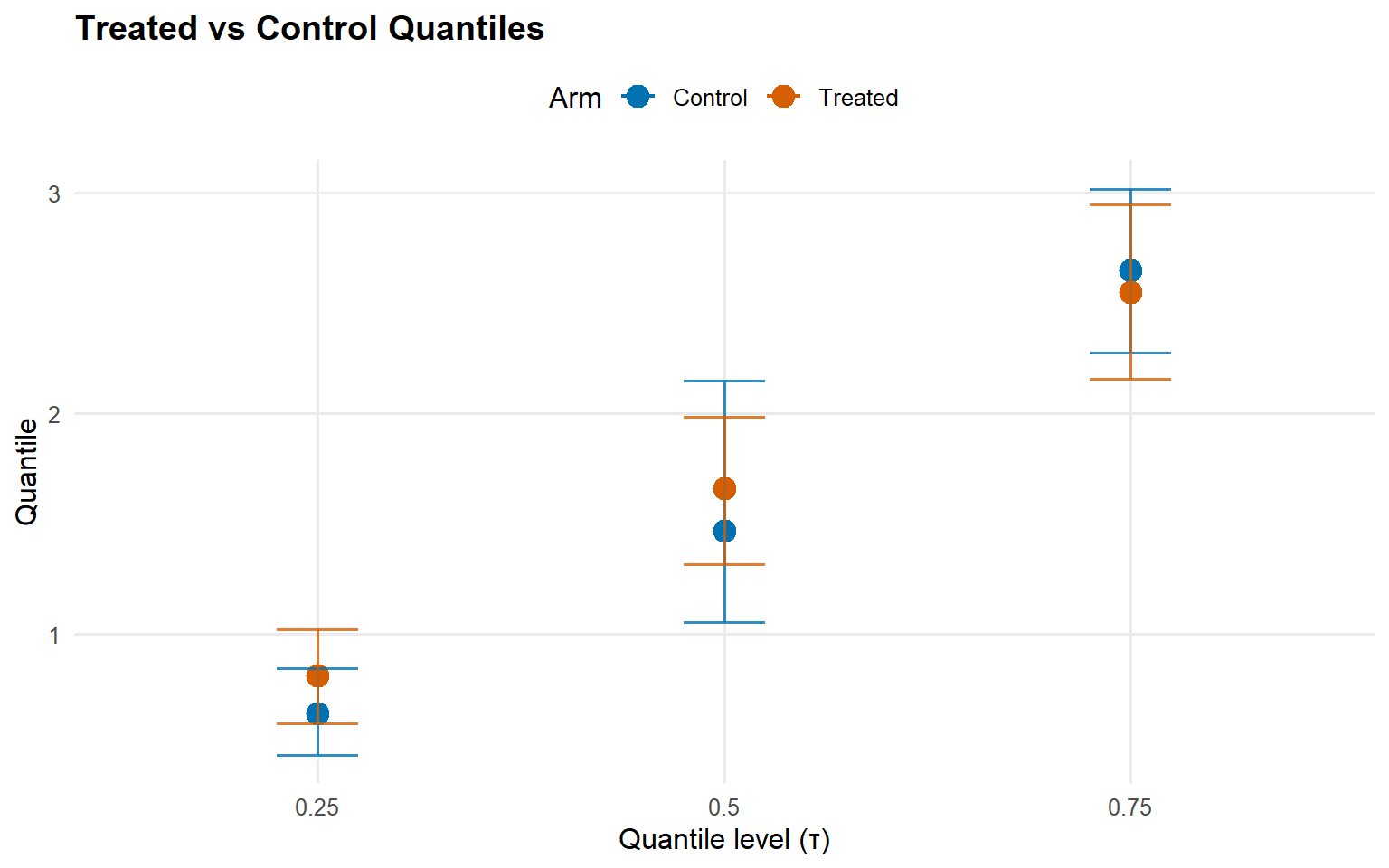
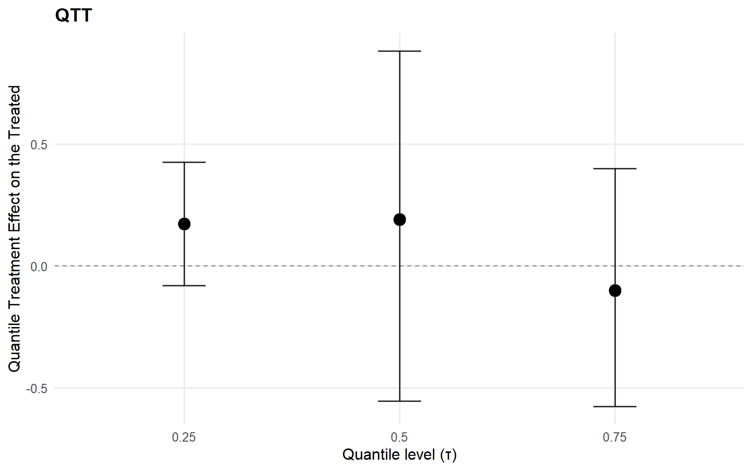
  index    estimate       lower     upper
1  0.25  0.17270432 -0.07889603 0.4250001
2  0.50  0.19139716 -0.55257196 0.8816509
3  0.75 -0.09985004 -0.57517407 0.3992333

$fit_df
  index    estimate       lower     upper
1  0.25  0.17270432 -0.07889603 0.4250001
2  0.50  0.19139716 -0.55257196 0.8816509
3  0.75 -0.09985004 -0.57517407 0.3992333

$lower
[1] -0.07889603 -0.55257196 -0.57517407

$upper
[1] 0.4250001 0.8816509 0.3992333

$qte
$qte$fit
  index    estimate       lower     upper
1  0.25  0.17270432 -0.07889603 0.4250001
2  0.50  0.19139716 -0.55257196 0.8816509
3  0.75 -0.09985004 -0.57517407 0.3992333

$qte$draws
, , 1

               [,1]
 [1,]  0.1287629791
 [2,] -0.1332456252
 [3,]  0.0303336012
 [4,] -0.0184126278
 [5,] -0.0193407294
 [6,] -0.0343073323
 [7,]  0.0086856266
 [8,]  0.2455021374
 [9,]  0.1937363934
[10,]  0.2587364507
[11,]  0.1832300251
[12,]  0.2060050759
[13,]  0.2342316412
[14,]  0.2240440824
[15,]  0.2610187324
[16,]  0.2865283574
[17,]  0.3270466410
[18,]  0.3523919852
[19,]  0.3738278154
[20,]  0.2559115494
[21,]  0.1774994291
[22,]  0.1811404731
[23,]  0.0039228043
[24,]  0.2912818762
[25,]  0.0946364319
[26,]  0.1387677086
[27,]  0.0426923925
[28,] -0.0618880886
[29,] -0.0942841633
[30,]  0.0393527873
[31,]  0.1506993825
[32,]  0.1773688647
[33,]  0.2827492349
[34,]  0.3048613636
[35,]  0.1878716395
[36,]  0.0001280459
[37,]  0.0259096352
[38,]  0.0328451108
[39,] -0.0611695272
[40,]  0.1811980530
[41,]  0.3195630237
[42,]  0.1904094799
[43,] -0.0085487156
[44,]  0.3017957765
[45,]  0.3263986781
[46,]  0.0095750997
[47,] -0.0152571492
[48,]  0.3283926775
[49,]  0.4406240698
[50,]  0.3539425185
[51,]  0.3674717267
[52,]  0.1909473598
[53,]  0.4164770600
[54,]  0.3959569032
[55,]  0.3654314617
[56,]  0.1348144967
[57,]  0.1495632509
[58,] -0.0027853762
[59,]  0.4327113775
[60,]  0.2045050004

, , 2

             [,1]
 [1,] -0.05661537
 [2,] -0.38296149
 [3,]  0.18046696
 [4,]  0.07126461
 [5,]  0.02666179
 [6,] -0.37718641
 [7,] -0.35336540
 [8,]  0.59679425
 [9,]  0.38786398
[10,]  0.59178232
[11,]  0.55829702
[12,]  0.48718922
[13,]  0.53481636
[14,]  0.51472751
[15,]  0.64403570
[16,]  0.48734074
[17,]  0.52672166
[18,]  0.38109749
[19,]  0.53765255
[20,]  0.31192325
[21,]  0.03260523
[22,]  0.16571383
[23,]  0.35600833
[24,]  0.25736513
[25,]  0.49431465
[26,]  0.27350717
[27,] -0.09735138
[28,] -0.12642415
[29,] -0.59498826
[30,] -0.60338652
[31,] -0.24120519
[32,]  0.11931928
[33,]  0.20452304
[34,]  0.29077214
[35,] -0.17550763
[36,] -0.16904331
[37,] -0.26575729
[38,]  0.02990274
[39,] -0.44058177
[40,] -0.21021453
[41,] -0.08347455
[42,]  0.02607906
[43,] -0.50569079
[44,] -0.01409299
[45,]  0.36588857
[46,]  0.09086234
[47,] -0.08357356
[48,]  0.38926359
[49,]  0.51426764
[50,]  0.50679719
[51,]  0.75059088
[52,]  0.03744930
[53,]  0.94098923
[54,]  0.88477862
[55,]  0.68018352
[56,]  0.24615700
[57,]  0.16264838
[58,] -0.04916649
[59,]  0.87819404
[60,]  0.77760011

, , 3

               [,1]
 [1,] -0.4156390441
 [2,] -0.3979544016
 [3,]  0.1864923993
 [4,] -0.1158334980
 [5,] -0.2543406067
 [6,] -0.1533826190
 [7,] -0.0835053305
 [8,] -0.0238024246
 [9,] -0.1372273029
[10,] -0.0845652455
[11,]  0.2473862975
[12,] -0.1541927597
[13,]  0.0642517269
[14,]  0.0394808504
[15,] -0.2203044377
[16,] -0.5503861385
[17,]  0.0821251880
[18,] -0.0671572545
[19,] -0.2722840432
[20,]  0.0239177199
[21,] -0.3788684946
[22,] -0.1698056531
[23,] -0.0621853727
[24,] -0.1756100103
[25,] -0.1738214783
[26,] -0.1889882676
[27,] -0.0759817333
[28,] -0.0098277802
[29,] -0.5976012457
[30,] -0.5044798468
[31,] -0.3197143548
[32,]  0.0435991303
[33,] -0.0102651298
[34,] -0.0973713251
[35,] -0.0775018136
[36,] -0.1905600132
[37,] -0.1390878377
[38,] -0.2466176731
[39,] -0.4358974768
[40,] -0.4885181643
[41,]  0.0612279426
[42,] -0.0068211441
[43,] -0.7174678578
[44,] -0.1307587403
[45,]  0.1632387303
[46,] -0.0002681153
[47,] -0.3939357136
[48,]  0.2191277678
[49,]  0.3303920445
[50,]  0.0363143711
[51,]  0.2520918968
[52,]  0.2350462384
[53,]  0.0403480683
[54,]  0.3874045624
[55,]  0.0956619237
[56,] -0.1702222530
[57,] -0.1431654327
[58,] -0.5296427806
[59,]  0.4099355421
[60,]  0.4565157643



$probs
[1] 0.25 0.50 0.75

Code

plot(qtt_gpd)

Model B: SB Bulk-only (Amoroso)

Code

bundle_sb_bulk <- bundle(
  y = y,
  treat = A,
  X = X,
  kernel = "amoroso",
  backend = "sb",
  PS = FALSE,
  GPD = FALSE,
  components = components_ex10,
  mcmc_outcome = bulk_mcmc_ex10
)

bundle_sb_bulk

CausalMixGPD causal bundle
PS model: disabled 
      Field                Treated                Control
    Backend Stick-Breaking Process Stick-Breaking Process
     Kernel                amoroso                amoroso
 Components                      3                      3
   GPD tail                  FALSE                  FALSE
    Epsilon                  0.025                  0.025

Outcome PS included: FALSE 
n (control) = 232 | n (treated) = 268

Code

fit_sb_bulk <- load_or_fit(
  tag_sb_bulk_ex10,
  quiet_mcmc(dpmix.causal(bundle_sb_bulk, mcmc = causal_run_mcmc_bulk))
)
summary(fit_sb_bulk)


-- Outcome fits --
[control]
MixGPD summary | backend: Stick-Breaking Process | kernel: Amoroso Distribution | GPD tail: FALSE | epsilon: 0.025
n = 232 | components = 3
Summary
Initial components: 3 | Components after truncation: 3

Summary table
       parameter   mean    sd q0.025 q0.500 q0.975
      weights[1]    0.5 0.032  0.488  0.488  0.585
      weights[2]  0.289 0.038  0.213  0.308  0.321
      weights[3]  0.211 0.025  0.191  0.202  0.254
           alpha  1.255 0.747  0.403  1.145  2.718
       shape1[1]    0.9 0.132   0.77   0.87  1.147
       shape1[2]  2.171 0.323   1.74  2.187  2.947
       shape1[3]  3.332 0.621  2.338  3.366  4.378
       shape2[1]  1.185 0.173  0.927  1.236  1.429
       shape2[2]  1.299 0.401  1.093  1.216  3.138
       shape2[3]  2.942 0.446  1.216  3.085  3.248
   beta_loc[1,1]      0     0      0      0      0
   beta_loc[1,2]      0     0      0      0      0
   beta_loc[1,3]      0     0      0      0      0
   beta_loc[1,4]      0     0      0      0      0
   beta_loc[2,1]      0     0      0      0      0
   beta_loc[2,2]      0     0      0      0      0
   beta_loc[2,3]      0     0      0      0      0
   beta_loc[2,4]      0     0      0      0      0
   beta_loc[3,1]      0     0      0      0      0
   beta_loc[3,2]      0     0      0      0      0
   beta_loc[3,3]      0     0      0      0      0
   beta_loc[3,4]      0     0      0      0      0
 beta_scale[1,1] -0.031 0.134 -0.336  -0.02   0.21
 beta_scale[1,2] -0.305 0.222 -0.694  -0.31   0.17
 beta_scale[1,3] -0.059 0.126 -0.267  -0.07   0.21
 beta_scale[1,4]  0.172 0.391 -0.545  0.226  0.748
 beta_scale[2,1]   0.21 0.177 -0.119  0.192  0.672
 beta_scale[2,2]  0.342 0.208 -0.078  0.326  0.762
 beta_scale[2,3] -0.048 0.088 -0.206 -0.051  0.085
 beta_scale[2,4] -0.169 0.385 -1.062 -0.177  0.528
 beta_scale[3,1] -0.127 0.073 -0.244 -0.137  0.088
 beta_scale[3,2] -0.099 0.118 -0.225 -0.127  0.269
 beta_scale[3,3]  0.034 0.069 -0.111  0.045  0.152
 beta_scale[3,4]  0.414 0.211  -0.39  0.448  0.681

[treated]
MixGPD summary | backend: Stick-Breaking Process | kernel: Amoroso Distribution | GPD tail: FALSE | epsilon: 0.025
n = 268 | components = 3
Summary
Initial components: 3 | Components after truncation: 3

Summary table
       parameter   mean    sd q0.025 q0.500 q0.975
      weights[1]  0.431 0.029   0.39  0.429  0.489
      weights[2]  0.381 0.011  0.352  0.389  0.389
      weights[3]  0.188 0.036  0.122  0.194  0.257
           alpha  1.649 0.735  0.255  1.513  3.229
       shape1[1]  1.407 0.374  0.913  1.271  2.191
       shape1[2]  2.141 0.306  1.095  2.221  2.462
       shape1[3]  1.726 0.457   1.05   1.91  2.308
       shape2[1]  1.383 0.134  1.189    1.4  1.715
       shape2[2]  1.495 0.121  1.393    1.5  1.883
       shape2[3]  0.853 0.077   0.69   0.87  0.954
   beta_loc[1,1]      0     0      0      0      0
   beta_loc[1,2]      0     0      0      0      0
   beta_loc[1,3]      0     0      0      0      0
   beta_loc[1,4]      0     0      0      0      0
   beta_loc[2,1]      0     0      0      0      0
   beta_loc[2,2]      0     0      0      0      0
   beta_loc[2,3]      0     0      0      0      0
   beta_loc[2,4]      0     0      0      0      0
   beta_loc[3,1]      0     0      0      0      0
   beta_loc[3,2]      0     0      0      0      0
   beta_loc[3,3]      0     0      0      0      0
   beta_loc[3,4]      0     0      0      0      0
 beta_scale[1,1]  0.021 0.143  -0.24   0.03  0.252
 beta_scale[1,2]  0.109 0.277 -0.416  0.136  0.567
 beta_scale[1,3] -0.123 0.188 -0.376 -0.169    0.3
 beta_scale[1,4]  0.253  0.22 -0.079  0.254  0.637
 beta_scale[2,1] -0.087  0.09 -0.236 -0.089  0.118
 beta_scale[2,2] -0.171 0.307 -0.542 -0.252  0.661
 beta_scale[2,3]    0.3 0.185 -0.179  0.346  0.534
 beta_scale[2,4]  0.158 0.144 -0.117  0.137  0.565
 beta_scale[3,1]  0.029 0.385 -0.604 -0.012  0.778
 beta_scale[3,2]   -0.1 0.478 -0.944 -0.128  0.792
 beta_scale[3,3] -0.042 0.257 -0.518 -0.003  0.425
 beta_scale[3,4] -0.871 0.695 -2.075 -0.843  0.363

Code

pred_mean_bulk <- predict(fit_sb_bulk, newdata =x_eval, type = "mean", interval = "credible", nsim_mean = nsim_mean_ex10, workers = predict_workers_ex10)
head(pred_mean_bulk)

  id    estimate       lower        upper ps
1  1 0.018796788 -0.04220241 -0.054109015 NA
2  2 0.220257543  0.19060980  0.238670583 NA
3  3 0.009106138  0.13795207 -0.086632614 NA
4  4 0.250474778  0.33353061  0.366750593 NA
5  5 0.623733045  0.47954650  0.917300205 NA
6  6 0.006877309  0.01167569 -0.009368928 NA

Code

plot(pred_mean_bulk)

Code

pred_q_bulk <- predict(fit_sb_bulk, newdata =x_eval, type = "quantile", p = 0.5, interval = "credible", workers = predict_workers_ex10)
head(pred_q_bulk)

  id index    estimate      lower     upper ps
1  1   0.5 -0.07632893 -0.4371972 0.3490505 NA
2  2   0.5  0.07230318 -0.3065777 0.4840868 NA
3  3   0.5  0.04028022 -0.1748914 0.2791915 NA
4  4   0.5  0.18537734 -0.1436805 0.4759454 NA
5  5   0.5  0.34618415 -0.1809036 0.8818743 NA
6  6   0.5 -0.09990753 -0.3474807 0.1673068 NA

Code

plot(pred_q_bulk)

Code

pred_d_bulk <- predict(fit_sb_bulk, newdata =x_eval, y = y_eval, type = "density", interval = "credible", workers = predict_workers_ex10)
head(pred_d_bulk)

  id         y ps trt_estimate  trt_lower trt_upper con_estimate  con_lower
1  1 0.9001906 NA            1 0.39768819 0.6786124            1 0.29903935
2  2 1.3517565 NA            2 0.24388238 0.4881761            2 0.21057718
3  3 1.1475287 NA            3 0.45632334 0.5798971            3 0.37361634
4  4 1.9323578 NA            4 0.21313001 0.3490534            4 0.13538138
5  5 3.3439817 NA            5 0.06210731 0.1521166            5 0.01648154
6  6 0.9493979 NA            6 0.44165049 0.5665514            6 0.27559040
   con_upper
1 0.43169610
2 0.50669354
3 0.61532199
4 0.40986958
5 0.07097451
6 0.42247395

Code

plot(pred_d_bulk)

Code

pred_surv_bulk <- predict(fit_sb_bulk, newdata =x_eval, y = y_eval, type = "survival", interval = "credible", workers = predict_workers_ex10)
head(pred_surv_bulk)

  id         y ps trt_estimate trt_lower trt_upper con_estimate  con_lower
1  1 0.9001906 NA            1 0.5482779 0.7653811            1 0.54222635
2  2 1.3517565 NA            2 0.4270570 0.6136765            2 0.40147708
3  3 1.1475287 NA            3 0.4348044 0.5973510            3 0.40647107
4  4 1.9323578 NA            4 0.2270964 0.3952450            4 0.09544257
5  5 3.3439817 NA            5 0.0474621 0.3106530            5 0.01193598
6  6 0.9493979 NA            6 0.5655855 0.7037081            6 0.53826126
  con_upper
1 0.7254776
2 0.6026171
3 0.5937754
4 0.2928773
5 0.1532955
6 0.6992092

Code

plot(pred_surv_bulk)

Code

cate_bulk <- cate(fit_sb_bulk, newdata = x_eval, interval = "credible", nsim_mean = nsim_mean_ex10)
head(format_cate_table(cate_bulk))

  id index    estimate       lower     upper
1  1     1 0.018796788 -0.47866010 0.4387606
2  2     1 0.220257543 -0.19853405 0.6999444
3  3     1 0.009106138 -0.40763481 0.4775009
4  4     1 0.250474778 -0.16551352 0.8009572
5  5     1 0.623733045 -0.09514537 1.5117428
6  6     1 0.006877309 -0.24431407 0.3080974

Code

plot(cate_bulk)

Code

cqte_bulk <- cqte(fit_sb_bulk, probs = c(0.25, 0.5, 0.75), newdata = x_eval, interval = "credible")
head(format_cqte_table(cqte_bulk))

  id index    estimate      lower     upper
1  1     1  0.10873915 -0.1756041 0.3722602
2  1     2 -0.07632893 -0.4371972 0.3490505
3  1     3 -0.15646853 -0.7383346 0.3753857
4  2     1  0.10525782 -0.2434054 0.4828703
5  2     2  0.07230318 -0.3065777 0.4840868
6  2     3  0.26761938 -0.2893173 1.0024245

Code

plot(cqte_bulk)

Prereqs

Required packages and data for this page are listed in the setup chunks above.

Outputs

This page renders model fits, diagnostics, and summary artifacts generated by package APIs.

Interpretation

Canonical concept page: 03 Causal Inference Objects
Treat this page as an application/example view and use the canonical page for core definitions.

Continue to the linked canonical concept page, then return for implementation-specific details.

ex10. Causal (X, no PS, SB Backend) - InvGauss/Amoroso

Causal Inference: X Without PS (CRP+SB)

What you’ll learn

When to use this template

Key limitation (important)

What this page does

Data Setup

Model A: CRP with GPD Tail (InvGauss)

Model B: SB Bulk-only (Amoroso)

Workflow Navigation

Prereqs

Outputs

Interpretation

Next