ex11. Causal (Same backend, CRP Backend) - Laplace Kernel

Website workflow note. This page reflects the current exported API and recommended wrapper-first usage. Last updated: 2026-02-19.

For the full package narrative, see the main package vignettes (basic, unconditional, conditional, and causal).

Causal Inference: Same Backend (CRP) - Laplace Kernel

This vignette fits two CRP-based causal models using the same kernel (Laplace):

Model A: bulk-only outcome models (GPD = FALSE)
Model B: GPD-augmented outcome models (GPD = TRUE)

Each model demonstrates the standard causal S3 workflow: bundle, fit, predict, plot, ATE, and QTE.

What you’ll learn

How to hold backend and kernel fixed and isolate the impact of tail augmentation.
How tail augmentation can change upper-quantile behavior even when mean effects look similar.
How to run the standard causal post-fit workflow for multiple estimands.

When to use this template

You want a clean sensitivity check focused on tail modeling rather than backend or kernel changes.
You want predictable runtime and an explicit complexity knob (components) inside a causal workflow.

Next steps

Compare this page with the SB version to study how tail augmentation behaves under a different backend.

Data Setup

Code

data("causal_alt_real500_p4_k2")
y <- causal_alt_real500_p4_k2$y
A <- causal_alt_real500_p4_k2$A
X <- as.matrix(causal_alt_real500_p4_k2$X)

summary_tbl <- tibble(
  statistic = c("N", "Mean", "SD", "Min", "Max"),
  value = c(length(y), mean(y), sd(y), min(y), max(y))
)

summary_tbl

# A tibble: 5 × 2
  statistic   value
  <chr>       <dbl>
1 N         500    
2 Mean        0.274
3 SD          1.76 
4 Min        -8.09 
5 Max         5.27

Code

x_eval <- X[seq_len(if (isTRUE(FAST)) 20L else 40L), , drop = FALSE]
y_eval <- y[seq_len(if (isTRUE(FAST)) 20L else 40L)]
u_threshold <- as.numeric(stats::quantile(y, 0.8, names = FALSE))

Code

df_causal <- data.frame(y = y, A = as.factor(A), x1 = X[, 1], x2 = X[, 2])

p_scatter <- ggplot(df_causal, aes(x = x1, y = y, color = A)) +
  geom_point(alpha = 0.5) +
  labs(title = "Outcome vs X1 by Treatment", x = "X1", y = "y", color = "Treatment") +
  theme_minimal()

p_scatter

Model A: CRP Bulk-only (Laplace)

Code

bundle_crp_bulk <- bundle(
  y = y,
  treat = A,
  X = X,
  kernel = "laplace",
  backend = "crp",
  PS = "logit",
  GPD = FALSE,
  components = components_ex11,
  mcmc_outcome = bulk_mcmc_ex11,
  mcmc_ps = mcmc_ps_bulk_ex11
)

bundle_crp_bulk

CausalMixGPD causal bundle
PS model: Bayesian logit (A | X) 
      Field                    Treated                    Control
    Backend Chinese Restaurant Process Chinese Restaurant Process
     Kernel                    laplace                    laplace
 Components                          3                          3
   GPD tail                      FALSE                      FALSE
    Epsilon                      0.025                      0.025

Outcome PS included: TRUE 
n (control) = 232 | n (treated) = 268

Code

summary(bundle_crp_bulk)

CausalMixGPD causal bundle summary
CausalMixGPD causal bundle
PS model: Bayesian logit (A | X) 
      Field                    Treated                    Control
    Backend Chinese Restaurant Process Chinese Restaurant Process
     Kernel                    laplace                    laplace
 Components                          3                          3
   GPD tail                      FALSE                      FALSE
    Epsilon                      0.025                      0.025

Outcome PS included: TRUE 
n (control) = 232 | n (treated) = 268

Code

fit_crp_bulk <- load_or_fit(
  tag_crp_bulk_ex11,
  quiet_mcmc(dpmix.causal(bundle_crp_bulk, mcmc = causal_run_mcmc_bulk))
)
summary(fit_crp_bulk)

-- PS fit --
CausalMixGPD PS fit summary
model: logit 
n = 500 | predictors = 5
Monitors: beta 

Summary table
 parameter   mean    sd q0.025 q0.500 q0.975
   beta[1]  0.031 0.186 -0.234 -0.009  0.456
   beta[2]  0.463  0.13  0.168  0.524  0.646
   beta[3]   0.41 0.209  0.103  0.461   0.82
   beta[4] -0.185 0.075 -0.281 -0.117 -0.116
   beta[5]  0.235 0.305  -0.42  0.247   0.74

-- Outcome fits --
[control]
MixGPD summary | backend: Chinese Restaurant Process | kernel: Laplace Distribution | GPD tail: FALSE | epsilon: 0.025
n = 232 | components = 3
Summary
Initial components: 3 | Components after truncation: 3

WAIC: 877.95
lppd: -337.882 | pWAIC: 101.093

Summary table
          parameter   mean    sd q0.025 q0.500 q0.975
         weights[1]  0.445 0.059  0.359  0.435   0.59
         weights[2]   0.32 0.042  0.224  0.323  0.385
         weights[3]  0.235 0.041  0.165  0.237  0.306
              alpha  0.452 0.278  0.095   0.41  1.087
           scale[1]  1.012 0.143  0.813  0.997  1.363
           scale[2]  1.136 0.205  0.837  1.122  1.642
           scale[3]  1.286 0.299  0.853  1.287  1.901
 beta_location[1,1] -0.299 0.483 -0.848 -0.452  0.423
 beta_location[1,2]    0.5 0.731 -1.035  0.974  1.193
 beta_location[1,3] -0.245 0.142 -0.528 -0.232  0.124
 beta_location[1,4]  0.341 0.859 -1.089  0.455    1.8
 beta_location[2,1]  0.186 0.653 -0.787  0.423  0.994
 beta_location[2,2] -0.545 0.845 -1.808 -0.733  1.503
 beta_location[2,3] -0.333 0.405 -1.118 -0.393  0.379
 beta_location[2,4]  0.262 1.075 -1.118 -0.325  1.805
 beta_location[3,1] -0.321 0.416 -0.724 -0.411  0.733
 beta_location[3,2] -0.466 1.279  -1.76  -0.91  1.824
 beta_location[3,3]  0.027 0.424 -0.637  0.042   0.56
 beta_location[3,4]  1.267 0.884 -1.014  1.568  2.112

[treated]
MixGPD summary | backend: Chinese Restaurant Process | kernel: Laplace Distribution | GPD tail: FALSE | epsilon: 0.025
n = 268 | components = 3
Summary
Initial components: 3 | Components after truncation: 3

WAIC: 1080.221
lppd: -431.47 | pWAIC: 108.64

Summary table
          parameter   mean    sd q0.025 q0.500 q0.975
         weights[1]  0.513  0.06  0.415  0.506  0.641
         weights[2]  0.335 0.065  0.193  0.343  0.445
         weights[3]  0.151 0.044  0.053   0.16   0.22
              alpha  0.395 0.217  0.089  0.358  0.924
           scale[1]  0.728 0.088   0.58  0.727   0.91
           scale[2]  1.012 0.304  0.668  0.938  1.772
           scale[3]  2.456 1.519  0.808  2.196  5.816
 beta_location[1,1] -0.091 0.153 -0.334 -0.089  0.255
 beta_location[1,2] -0.673 1.594 -2.172 -1.402  1.887
 beta_location[1,3]  0.039  0.18 -0.238  0.012  0.422
 beta_location[1,4]  0.124 0.389 -0.455  0.172  0.711
 beta_location[2,1]  0.069 0.368 -0.831  0.115  0.475
 beta_location[2,2]  0.493 1.534 -2.017  1.132  1.958
 beta_location[2,3]  0.229   0.3 -0.251  0.207  0.867
 beta_location[2,4]  0.691 0.355  0.069  0.661  1.564
 beta_location[3,1]  0.026 0.428 -0.915  0.257  0.387
 beta_location[3,2]   1.63 0.345  1.005  1.557  2.704
 beta_location[3,3]  0.305 0.199  0.094  0.273  0.752
 beta_location[3,4]  0.824 0.352  0.299  0.866  1.652

Code

params(fit_crp_bulk)

Posterior mean parameters (causal)

[ps]
Posterior mean parameters

$beta
[1]  0.03087  0.46270  0.40980 -0.18530  0.23550

[treated]
Posterior mean parameters

$alpha
[1] 0.3954

$w
[1] 0.5135 0.3352 0.1513

$beta_location
      PropScore       x1      x2      x3     x4
comp1    0.4504 -0.09074 -0.6728 0.03941 0.1236
comp2   -0.0613  0.06893  0.4928 0.22880 0.6908
comp3   -0.2750  0.02585  1.6300 0.30460 0.8238

$scale
[1] 0.7281 1.0120 2.4560

[control]
Posterior mean parameters

$alpha
[1] 0.4518

$w
[1] 0.4448 0.3204 0.2348

$beta_location
      PropScore      x1      x2       x3     x4
comp1   0.54190 -0.2989  0.5001 -0.24490 0.3409
comp2  -0.62400  0.1860 -0.5454 -0.33340 0.2618
comp3  -0.02545 -0.3210 -0.4662  0.02667 1.2670

$scale
[1] 1.012 1.136 1.286

Code

plot(fit_crp_bulk, family = plot_family_bulk_ex11)


=== treated ===

=== traceplot ===


=== control ===

=== traceplot ===

Code

pred_mean_bulk <- predict(fit_crp_bulk, newdata = x_eval, type = "mean",
                          interval = "credible", nsim_mean = nsim_mean_ex11, workers = predict_workers_ex11)
head(pred_mean_bulk)

  id    estimate      lower       upper        ps
1  1 -0.68172173 -0.7967055 -0.43669055 0.4311567
2  2  0.26097700  0.4483003  0.07157906 0.6254685
3  3  0.02387166 -0.1538391  0.31510372 0.6559320
4  4  0.45654418  0.3056108  0.60190307 0.5880164
5  5  0.83009024  0.7119392  0.95146591 0.5079531
6  6 -0.46811388 -0.3666685 -0.46594988 0.5613561

Code

plot(pred_mean_bulk)

Code

pred_q_bulk <- predict(fit_crp_bulk, newdata = x_eval, type = "quantile",
                       p = 0.5, interval = "credible", workers = predict_workers_ex11)
head(pred_q_bulk)

  id index   estimate      lower        upper        ps
1  1   0.5 -0.3929639 -1.4728209  0.409633023 0.4311567
2  2   0.5  0.2946624 -0.3072996  0.814073279 0.6254685
3  3   0.5 -0.2009780 -0.8832226  0.635894380 0.6559320
4  4   0.5  0.2124528 -0.4622937  1.068710482 0.5880164
5  5   0.5  0.3765908 -1.0159254  2.217549656 0.5079531
6  6   0.5 -0.6176759 -1.2132896 -0.002148522 0.5613561

Code

plot(pred_q_bulk)

Code

pred_d_bulk <- predict(fit_crp_bulk, newdata = x_eval, y = y_eval,
                       type = "density", interval = "credible", workers = predict_workers_ex11)
head(pred_d_bulk)

  id          y        ps trt_estimate  trt_lower trt_upper con_estimate
1  1  0.8901906 0.4311567            1 0.08720809 0.3824647            1
2  2 -1.3417565 0.6254685            2 0.05864055 0.1479797            2
3  3  1.1375287 0.6559320            3 0.09138138 0.3801801            3
4  4 -1.9223578 0.5880164            4 0.04764998 0.1882130            4
5  5 -3.3339817 0.5079531            5 0.01358938 0.0957584            5
6  6  0.9393979 0.5613561            6 0.17178347 0.3289046            6
   con_lower con_upper
1 0.17731785 0.3525725
2 0.09419684 0.2807646
3 0.12667777 0.2316647
4 0.07152481 0.1372626
5 0.02099072 0.1158880
6 0.18487785 0.3865118

Code

plot(pred_d_bulk)

Code

pred_surv_bulk <- predict(fit_crp_bulk, newdata = x_eval, y = y_eval,
                          type = "survival", interval = "credible", workers = predict_workers_ex11)
head(pred_surv_bulk)

  id          y        ps trt_estimate trt_lower trt_upper con_estimate
1  1  0.8901906 0.4311567            1 0.2224514 0.5146740            1
2  2 -1.3417565 0.6254685            2 0.8721773 0.9439091            2
3  3  1.1375287 0.6559320            3 0.1327757 0.3660092            3
4  4 -1.9223578 0.5880164            4 0.8573525 0.9466908            4
5  5 -3.3339817 0.5079531            5 0.9280423 0.9863161            5
6  6  0.9393979 0.5613561            6 0.1796831 0.2906318            6
  con_lower con_upper
1 0.3185779 0.5248769
2 0.7299551 0.8984880
3 0.1297222 0.2453379
4 0.8394169 0.9329809
5 0.8098265 0.9787328
6 0.3212788 0.5486566

Code

plot(pred_surv_bulk)

Code

ate_bulk <- ate(fit_crp_bulk, interval = "credible", nsim_mean = nsim_mean_ex11)
head(ate_bulk)

$fit
[1] -0.04781558

$fit_df
     estimate      lower     upper
1 -0.04781558 -0.2740216 0.1922627

$lower
[1] -0.2740216

$upper
[1] 0.1922627

$ate
$ate$fit
     estimate      lower     upper
1 -0.04781558 -0.2740216 0.1922627

$ate$draws
              [,1]
 [1,]  0.030736411
 [2,]  0.065840194
 [3,]  0.108732953
 [4,]  0.108038197
 [5,]  0.108674932
 [6,]  0.121568188
 [7,]  0.100462338
 [8,] -0.004008413
 [9,] -0.039224495
[10,]  0.043146414
[11,]  0.015449635
[12,]  0.045183402
[13,] -0.019472243
[14,]  0.093583574
[15,]  0.194901500
[16,]  0.093267919
[17,] -0.108912621
[18,] -0.016647419
[19,] -0.093114472
[20,] -0.014779869
[21,] -0.015859619
[22,]  0.150039790
[23,]  0.176378888
[24,]  0.144991339
[25,] -0.051574900
[26,] -0.055071771
[27,] -0.029060321
[28,] -0.121293953
[29,] -0.142294665
[30,] -0.124821658
[31,] -0.201360972
[32,] -0.115663213
[33,] -0.065487511
[34,] -0.015924711
[35,] -0.059408186
[36,] -0.112461057
[37,] -0.008909915
[38,] -0.019897898
[39,] -0.169274685
[40,] -0.105043606
[41,] -0.090720952
[42,]  0.090980001
[43,] -0.168416818
[44,] -0.169065707
[45,] -0.155489837
[46,] -0.086797163
[47,] -0.133347258
[48,] -0.223598398
[49,] -0.241038378
[50,] -0.057258989
[51,] -0.100405952
[52,] -0.104028704
[53,] -0.197729121
[54,] -0.243047501
[55,] -0.173921227
[56,] -0.190301952
[57,] -0.310608550
[58,] -0.216380531
[59,] -0.199145752
[60,] -0.283014023
[61,] -0.352912140
[62,] -0.127228278
[63,] -0.103833172
[64,]  0.033086466
[65,] -0.053128502
[66,] -0.115983770
[67,] -0.086315295
[68,] -0.086763102
[69,] -0.104413714
[70,] -0.170630137
[71,] -0.051732489
[72,] -0.062175295
[73,] -0.087987125
[74,] -0.020428837
[75,] -0.116240222
[76,] -0.094996010
[77,] -0.061411499
[78,] -0.024594777
[79,]  0.077728627
[80,]  0.024473716
[81,]  0.016842932
[82,] -0.047746301
[83,] -0.223491850
[84,] -0.089755705
[85,] -0.058572026
[86,]  0.132793872
[87,]  0.385000181
[88,]  0.183173542
[89,]  0.246298600
[90,]  0.099449376


$grid
NULL

Code

plot(ate_bulk)

Code

qte_bulk <- qte(fit_crp_bulk, probs = c(0.25, 0.5, 0.75), interval = "credible")
head(qte_bulk)

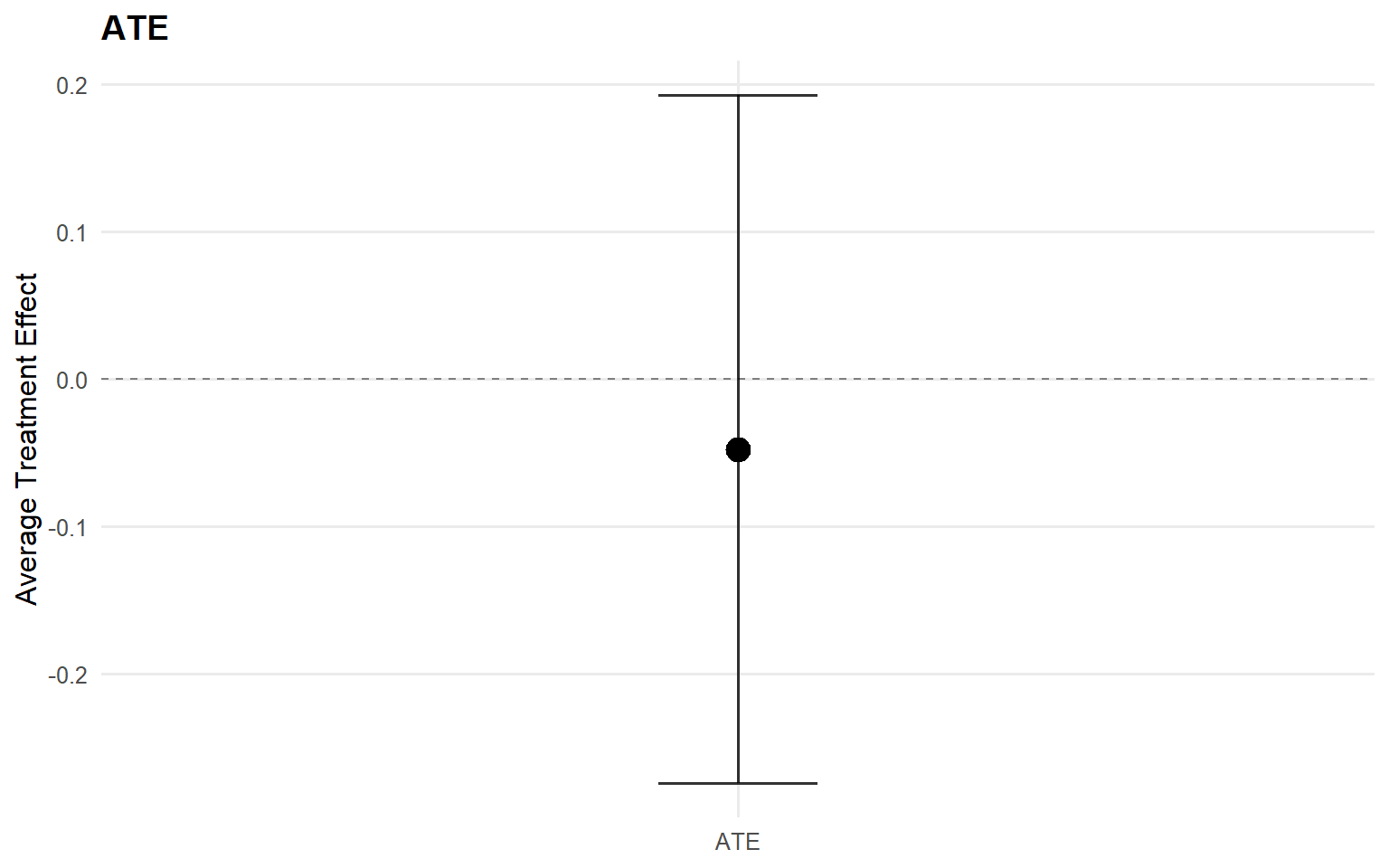
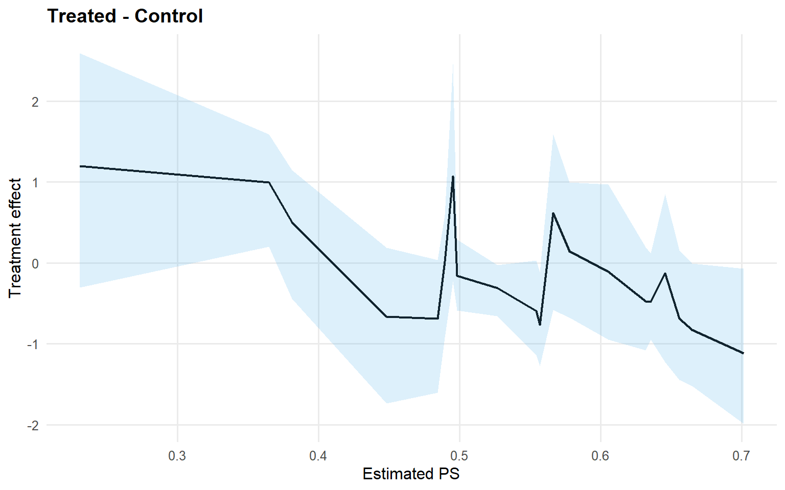
$fit
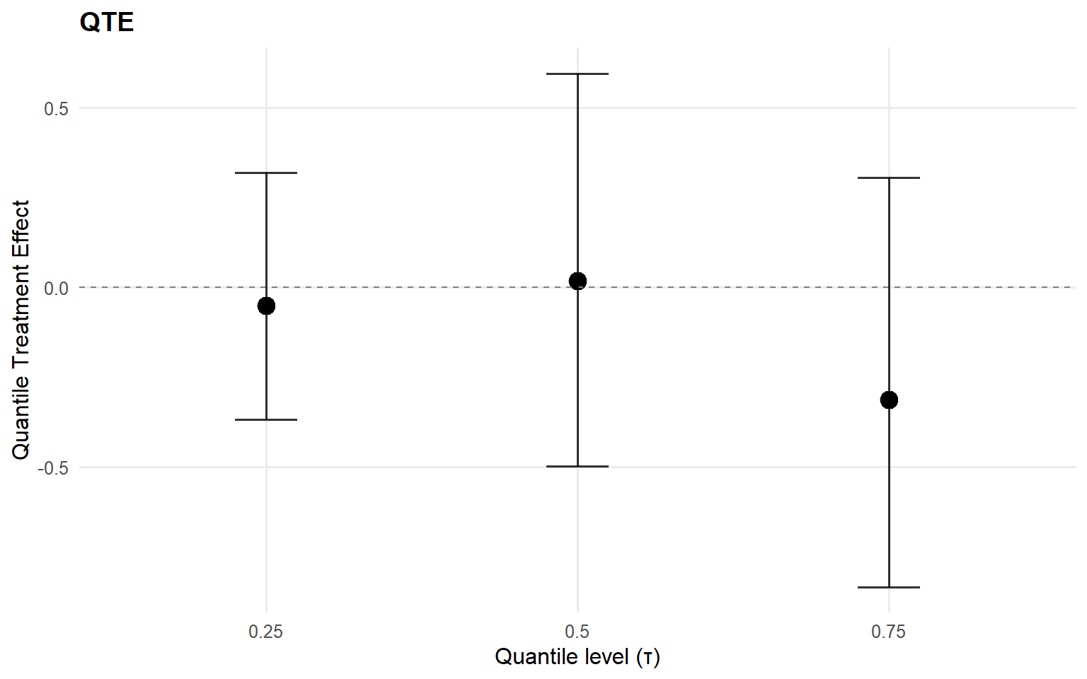
  index    estimate      lower     upper
1  0.25 -0.03453822 -0.4578704 0.3000317
2  0.50 -0.06214089 -0.4803350 0.3144029
3  0.75 -0.11304528 -0.7049802 0.4147881

$fit_df
  index    estimate      lower     upper
1  0.25 -0.03453822 -0.4578704 0.3000317
2  0.50 -0.06214089 -0.4803350 0.3144029
3  0.75 -0.11304528 -0.7049802 0.4147881

$lower
[1] -0.4578704 -0.4803350 -0.7049802

$upper
[1] 0.3000317 0.3144029 0.4147881

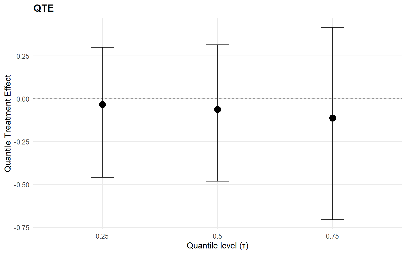
$qte
$qte$fit
  index    estimate      lower     upper
1  0.25 -0.03453822 -0.4578704 0.3000317
2  0.50 -0.06214089 -0.4803350 0.3144029
3  0.75 -0.11304528 -0.7049802 0.4147881

$qte$draws
, , 1

              [,1]
 [1,]  0.043709335
 [2,]  0.131132709
 [3,]  0.223139040
 [4,]  0.117772385
 [5,] -0.356922199
 [6,]  0.131853557
 [7,] -0.071811459
 [8,] -0.268375775
 [9,] -0.189619370
[10,]  0.020175368
[11,] -0.445303737
[12,] -0.279374656
[13,] -0.042429918
[14,] -0.233787449
[15,]  0.230592156
[16,]  0.128408519
[17,] -0.254115497
[18,]  0.083323483
[19,] -0.067695918
[20,] -0.284575899
[21,] -0.207634706
[22,]  0.135321424
[23,]  0.152477120
[24,]  0.011546942
[25,] -0.130472065
[26,] -0.241793239
[27,] -0.015708168
[28,] -0.265357590
[29,] -0.112670495
[30,] -0.433802411
[31,] -0.351310280
[32,]  0.053355858
[33,]  0.444951931
[34,] -0.117841403
[35,]  0.130488639
[36,] -0.118774557
[37,]  0.038011868
[38,]  0.150523301
[39,] -0.123756943
[40,] -0.108957156
[41,]  0.030067292
[42,]  0.172131137
[43,] -0.104723073
[44,] -0.031876979
[45,] -0.040161736
[46,] -0.234373450
[47,] -0.296631797
[48,] -0.333291968
[49,] -0.716884129
[50,] -0.056477246
[51,]  0.016758376
[52,] -0.242433862
[53,] -0.020528307
[54,] -0.354413143
[55,] -0.104246822
[56,] -0.109817755
[57,] -0.461518842
[58,] -0.051546640
[59,] -0.061326124
[60,] -0.025922822
[61,] -0.305430651
[62,]  0.157299935
[63,]  0.213135433
[64,]  0.261618424
[65,] -0.235931321
[66,]  0.189187374
[67,]  0.065764865
[68,]  0.322942179
[69,]  0.236925413
[70,]  0.262666267
[71,]  0.227627831
[72,]  0.072452963
[73,] -0.035905719
[74,]  0.284279289
[75,]  0.198222762
[76,]  0.264292589
[77,]  0.117708391
[78,]  0.178460277
[79,]  0.194520420
[80,]  0.304605020
[81,]  0.158399487
[82,] -0.158591338
[83,] -0.493598675
[84,] -0.309140975
[85,] -0.005371278
[86,] -0.222657916
[87,]  0.263461308
[88,] -0.004638298
[89,]  0.142520254
[90,]  0.069260893

, , 2

              [,1]
 [1,] -0.065371036
 [2,]  0.122850097
 [3,]  0.138547360
 [4,] -0.027724289
 [5,]  0.207264000
 [6,]  0.175053598
 [7,]  0.027986521
 [8,] -0.016130181
 [9,] -0.076791362
[10,]  0.205566431
[11,] -0.119453679
[12,]  0.008763608
[13,]  0.130124422
[14,]  0.140328222
[15,]  0.401856484
[16,]  0.008393922
[17,]  0.132916654
[18,]  0.177798716
[19,] -0.005123042
[20,]  0.005964241
[21,]  0.012415567
[22,]  0.195577178
[23,]  0.323908706
[24,]  0.074032983
[25,] -0.240974434
[26,] -0.020079897
[27,]  0.045370100
[28,] -0.358455773
[29,] -0.127090303
[30,] -0.264249075
[31,] -0.291660631
[32,]  0.024944847
[33,]  0.263351387
[34,] -0.062925761
[35,]  0.263648953
[36,]  0.029644997
[37,]  0.281660675
[38,]  0.074463447
[39,] -0.267513576
[40,] -0.115188857
[41,] -0.099831722
[42,]  0.177389597
[43,] -0.292281724
[44,] -0.141140938
[45,]  0.052752714
[46,] -0.128914176
[47,] -0.322449261
[48,] -0.379400372
[49,] -0.484852105
[50,] -0.146664139
[51,] -0.012908775
[52,] -0.194473472
[53,] -0.247253347
[54,] -0.344647872
[55,] -0.332726347
[56,] -0.172702873
[57,] -0.541544732
[58,] -0.275711458
[59,] -0.184467309
[60,] -0.206013791
[61,] -0.511302527
[62,] -0.032871555
[63,] -0.083448788
[64,]  0.005566095
[65,] -0.144513366
[66,] -0.034712794
[67,] -0.188705044
[68,] -0.055884054
[69,] -0.034566013
[70,] -0.164218293
[71,]  0.020301461
[72,]  0.006626609
[73,] -0.221535353
[74,] -0.068373365
[75,] -0.253423434
[76,] -0.301155738
[77,] -0.196817249
[78,] -0.088412120
[79,] -0.044244479
[80,] -0.091236139
[81,] -0.045118855
[82,] -0.069462382
[83,] -0.464776006
[84,] -0.162245798
[85,] -0.061906723
[86,] -0.083088362
[87,]  0.379617788
[88,]  0.100597913
[89,]  0.202037154
[90,] -0.041267986

, , 3

              [,1]
 [1,]  0.125069433
 [2,] -0.079291958
 [3,]  0.061382307
 [4,] -0.117071563
 [5,]  0.194923252
 [6,]  0.204081390
 [7,]  0.090941193
 [8,] -0.047887378
 [9,]  0.168778281
[10,]  0.036549058
[11,] -0.114063686
[12,]  0.053409353
[13,]  0.167271594
[14,]  0.320082267
[15,]  0.563068683
[16,] -0.132445704
[17,]  0.209597579
[18,]  0.278072982
[19,]  0.262074233
[20,]  0.219877820
[21,] -0.023930233
[22,]  0.431074409
[23,]  0.153968020
[24,]  0.232282882
[25,] -0.252403904
[26,] -0.040640694
[27,] -0.040006720
[28,] -0.464171648
[29,] -0.163507798
[30,] -0.197037966
[31,] -0.290749321
[32,] -0.105609197
[33,]  0.079741373
[34,]  0.004690825
[35,]  0.107356497
[36,] -0.140186687
[37,] -0.142708648
[38,]  0.036974408
[39,] -0.260562471
[40,] -0.350733344
[41,] -0.270009885
[42,]  0.060835676
[43,] -0.425195834
[44,] -0.283117511
[45,] -0.077086537
[46,] -0.336163228
[47,] -0.315834660
[48,] -0.218022803
[49,] -0.178871011
[50,]  0.194201492
[51,]  0.068150430
[52,]  0.062875725
[53,] -0.359905515
[54,] -0.480115959
[55,] -0.450091094
[56,] -0.201264587
[57,] -0.759053712
[58,] -0.316013618
[59,] -0.302979285
[60,] -0.566736815
[61,] -0.712534115
[62,] -0.239377109
[63,] -0.192689151
[64,] -0.001776688
[65,] -0.296017567
[66,] -0.496354453
[67,] -0.435859943
[68,] -0.153837323
[69,] -0.168944004
[70,] -0.416789638
[71,] -0.240833829
[72,] -0.121197377
[73,] -0.314002097
[74,] -0.678961025
[75,] -0.657219819
[76,] -0.758419706
[77,] -0.371974035
[78,] -0.107933092
[79,] -0.159657643
[80,]  0.022188070
[81,]  0.086352292
[82,] -0.041552097
[83,] -0.284751662
[84,] -0.068537057
[85,] -0.025491238
[86,]  0.358690819
[87,]  0.438239729
[88,]  0.034547195
[89,]  0.119477967
[90,] -0.172721132



$probs
[1] 0.25 0.50 0.75

Code

plot(qte_bulk)

Model B: CRP with GPD Tail (Laplace)

Code

param_specs_gpd <- list(
  gpd = list(
    threshold = list(
      mode = "dist",
      dist = "lognormal",
      args = list(meanlog = log(max(u_threshold, .Machine$double.eps)), sdlog = 0.25)
    )
  )
)

bundle_crp_gpd <- bundle(
  y = y,
  treat = A,
  X = X,
  kernel = "laplace",
  backend = "crp",
  PS = "logit",
  GPD = TRUE,
  components = components_ex11,
  param_specs = param_specs_gpd,
  mcmc_outcome = gpd_mcmc_ex11,
  mcmc_ps = mcmc_ps_gpd_ex11
)

bundle_crp_gpd

CausalMixGPD causal bundle
PS model: Bayesian logit (A | X) 
      Field                    Treated                    Control
    Backend Chinese Restaurant Process Chinese Restaurant Process
     Kernel                    laplace                    laplace
 Components                          3                          3
   GPD tail                       TRUE                       TRUE
    Epsilon                      0.025                      0.025

Outcome PS included: TRUE 
n (control) = 232 | n (treated) = 268

Code

summary(bundle_crp_gpd)

CausalMixGPD causal bundle summary
CausalMixGPD causal bundle
PS model: Bayesian logit (A | X) 
      Field                    Treated                    Control
    Backend Chinese Restaurant Process Chinese Restaurant Process
     Kernel                    laplace                    laplace
 Components                          3                          3
   GPD tail                       TRUE                       TRUE
    Epsilon                      0.025                      0.025

Outcome PS included: TRUE 
n (control) = 232 | n (treated) = 268

Code

fit_crp_gpd <- load_or_fit(
  tag_crp_gpd_ex11,
  quiet_mcmc(dpmgpd.causal(bundle_crp_gpd, mcmc = causal_run_mcmc_gpd))
)
summary(fit_crp_gpd)

-- PS fit --
CausalMixGPD PS fit summary
model: logit 
n = 500 | predictors = 5
Monitors: beta 

Summary table
 parameter   mean    sd q0.025 q0.500 q0.975
   beta[1]  0.021 0.082 -0.056 -0.005  0.144
   beta[2]  0.458 0.082  0.324  0.451  0.607
   beta[3]   0.27 0.197 -0.042  0.216  0.544
   beta[4] -0.149 0.065 -0.303 -0.107  -0.07
   beta[5]  0.277 0.149 -0.228  0.348   0.48

-- Outcome fits --
[control]
MixGPD summary | backend: Chinese Restaurant Process | kernel: Laplace Distribution | GPD tail: TRUE | epsilon: 0.025
n = 232 | components = 3
Summary
Initial components: 3 | Components after truncation: 2

WAIC: 904.477
lppd: -383.202 | pWAIC: 69.037

Summary table
          parameter   mean    sd q0.025 q0.500 q0.975
         weights[1]  0.641 0.114  0.496  0.634  0.869
         weights[2]  0.339 0.119  0.101   0.36  0.496
              alpha  0.408 0.276  0.044  0.324  0.908
 beta_tail_scale[1]  0.372 0.193  0.068  0.366    0.7
 beta_tail_scale[2]  0.203 0.208 -0.163  0.194  0.522
 beta_tail_scale[3] -0.018 0.202 -0.452 -0.026  0.366
 beta_tail_scale[4] -0.297 0.286 -0.722 -0.346  0.309
         tail_shape -0.065 0.089 -0.136 -0.123  0.097
          threshold  2.309 0.114  2.195   2.23   2.44
           scale[1]  1.196 0.197  0.913  1.169   1.72
           scale[2]  1.399  0.33  0.772  1.387  1.986
 beta_location[1,1]  0.386 0.309  0.108  0.257  1.212
 beta_location[1,2]   0.37 0.284  0.059  0.237  0.818
 beta_location[1,3] -0.501 0.264  -0.91 -0.511  0.003
 beta_location[1,4]  0.395  1.17 -0.637 -0.001  2.911
 beta_location[2,1]  0.493 0.542 -0.299  0.375  1.212
 beta_location[2,2]  0.226 0.624 -1.235  0.349  1.209
 beta_location[2,3] -0.181 0.299  -0.91 -0.061  0.096
 beta_location[2,4]  2.342   1.4 -0.525  2.761  4.318

[treated]
MixGPD summary | backend: Chinese Restaurant Process | kernel: Laplace Distribution | GPD tail: TRUE | epsilon: 0.025
n = 268 | components = 3
Summary
Initial components: 3 | Components after truncation: 3

WAIC: 1095.158
lppd: -447.506 | pWAIC: 100.073

Summary table
          parameter   mean    sd q0.025 q0.500 q0.975
         weights[1]  0.533 0.085  0.412  0.521  0.698
         weights[2]  0.274 0.057  0.158  0.274  0.388
         weights[3]  0.193 0.045  0.085   0.19  0.265
              alpha  0.453 0.238  0.107  0.411  0.975
 beta_tail_scale[1]  0.155 0.148 -0.113  0.154  0.445
 beta_tail_scale[2] -0.208 0.168 -0.509 -0.222  0.106
 beta_tail_scale[3]  0.075  0.14 -0.181  0.065  0.303
 beta_tail_scale[4] -0.217  0.25 -0.699 -0.236  0.278
         tail_shape -0.009 0.117 -0.146 -0.032  0.187
          threshold  1.813 0.128  1.435  1.822  2.093
           scale[1]  1.436 0.177  1.124  1.398  1.812
           scale[2]  1.191 0.336  0.653  1.162  1.823
           scale[3]  0.859 0.312   0.42  0.764  1.559
 beta_location[1,1]  0.378 0.173  0.172   0.43  0.649
 beta_location[1,2]  0.847 0.428  -0.42  0.841  1.331
 beta_location[1,3]  0.526 0.208  0.094  0.551  0.674
 beta_location[1,4]  0.417 0.318  0.083  0.408  1.203
 beta_location[2,1] -0.365 0.589 -1.284 -0.459  0.782
 beta_location[2,2] -1.111 1.088 -2.259 -1.468  1.167
 beta_location[2,3] -0.588 0.372 -1.283 -0.573  0.364
 beta_location[2,4]  0.891 0.914 -0.838  1.084  1.955
 beta_location[3,1] -0.436 0.242 -0.881 -0.391 -0.102
 beta_location[3,2]  0.044  0.92 -1.902   0.42  1.091
 beta_location[3,3] -0.417 0.266 -0.948 -0.487 -0.023
 beta_location[3,4] -0.183 1.005 -0.948 -0.684   2.36

Code

params(fit_crp_gpd)

Posterior mean parameters (causal)

[ps]
Posterior mean parameters

$beta
[1]  0.02086  0.45850  0.27050 -0.14870  0.27740

[treated]
Posterior mean parameters

$alpha
[1] 0.4532

$w
[1] 0.5333 0.2736 0.1931

$beta_location
      PropScore      x1       x2      x3      x4
comp1   0.14630  0.3779  0.84720  0.5256  0.4165
comp2   0.54640 -0.3655 -1.11100 -0.5879  0.8913
comp3  -0.07651 -0.4356  0.04363 -0.4169 -0.1826

$scale
[1] 1.436 1.191 0.859

$threshold
[1] 1.813

$beta_tail_scale
            x1      x2     x3      x4
overall 0.1554 -0.2081 0.0747 -0.2175

$tail_shape
[1] -0.009385

[control]
Posterior mean parameters

$alpha
[1] 0.4081

$w
[1] 0.6412 0.3393

$beta_location
      PropScore     x1     x2      x3     x4
comp1    -1.182 0.3864 0.3698 -0.5013 0.3947
comp2    -1.065 0.4925 0.2263 -0.1809 2.3420

$scale
[1] 1.196 1.399

$threshold
[1] 2.309

$beta_tail_scale
            x1     x2       x3      x4
overall 0.3723 0.2031 -0.01775 -0.2969

$tail_shape
[1] -0.06477

Code

plot(fit_crp_gpd, family = plot_family_gpd_ex11)


=== treated ===

=== density ===


=== control ===

=== density ===

Code

pred_mean_gpd <- predict(fit_crp_gpd, newdata = x_eval, type = "mean",
                         interval = "credible", nsim_mean = nsim_mean_ex11, workers = predict_workers_ex11)
head(pred_mean_gpd)

  id     estimate       lower       upper        ps
1  1 -0.566499479 -0.48289091 -0.95538040 0.4480745
2  2 -0.432027067 -0.01317664 -0.47830624 0.6454734
3  3 -0.606064603 -0.41427428 -0.81884756 0.6352615
4  4 -0.002837004  0.27194997 -0.05450042 0.5778090
5  5  0.609171821  0.59471767  0.60959331 0.4950231
6  6 -0.613531848 -0.52464508 -0.56934721 0.5542977

Code

plot(pred_mean_gpd)

Code

pred_q_gpd <- predict(fit_crp_gpd, newdata = x_eval, type = "quantile",
                      p = 0.5, interval = "credible", workers = predict_workers_ex11)
head(pred_q_gpd)

  id index   estimate      lower      upper        ps
1  1   0.5 -0.6636126 -1.7367542 0.18637478 0.4480745
2  2   0.5 -0.1266240 -1.2281784 0.84909686 0.6454734
3  3   0.5 -0.4780219 -0.9504982 0.12142176 0.6352615
4  4   0.5  0.1421048 -0.6760422 0.99461168 0.5778090
5  5   0.5  1.0697214 -0.2298549 2.46165460 0.4950231
6  6   0.5 -0.5928813 -1.1352213 0.03168954 0.5542977

Code

plot(pred_q_gpd)

Code

pred_d_gpd <- predict(fit_crp_gpd, newdata = x_eval, y = y_eval,
                      type = "density", interval = "credible", workers = predict_workers_ex11)
head(pred_d_gpd)

  id          y        ps trt_estimate  trt_lower trt_upper con_estimate
1  1  0.8901906 0.4480745            1 0.05347652 0.1747996            1
2  2 -1.3417565 0.6454734            2 0.11012104 0.2525614            2
3  3  1.1375287 0.6352615            3 0.15355558 0.2320959            3
4  4 -1.9223578 0.5778090            4 0.06939420 0.1751593            4
5  5 -3.3339817 0.4950231            5 0.03718816 0.1287411            5
6  6  0.9393979 0.5542977            6 0.12011584 0.2809338            6
   con_lower  con_upper
1 0.11591742 0.35348857
2 0.06938899 0.15104195
3 0.18455278 0.29230854
4 0.04757541 0.12318577
5 0.02381675 0.07505433
6 0.09107347 0.27640120

Code

plot(pred_d_gpd)

Code

pred_surv_gpd <- predict(fit_crp_gpd, newdata = x_eval, y = y_eval,
                         type = "survival", interval = "credible", workers = predict_workers_ex11)
head(pred_surv_gpd)

  id          y        ps trt_estimate trt_lower trt_upper con_estimate
1  1  0.8901906 0.4480745            1 0.2407669 0.3751256            1
2  2 -1.3417565 0.6454734            2 0.7279433 0.8667641            2
3  3  1.1375287 0.6352615            3 0.2037565 0.3172399            3
4  4 -1.9223578 0.5778090            4 0.7735803 0.9096077            4
5  5 -3.3339817 0.4950231            5 0.7688462 0.9560828            5
6  6  0.9393979 0.5542977            6 0.2469539 0.3995348            6
  con_lower con_upper
1 0.2321981 0.5474634
2 0.8055017 0.9309771
3 0.2277541 0.4994435
4 0.8491837 0.9446595
5 0.9091138 0.9707987
6 0.3531180 0.5283949

Code

plot(pred_surv_gpd)

Code

ate_gpd <- ate(fit_crp_gpd, interval = "credible", nsim_mean = nsim_mean_ex11)
head(ate_gpd)

$fit
[1] -0.2280586

$fit_df
    estimate      lower      upper
1 -0.2280586 -0.4529534 0.06953192

$lower
[1] -0.4529534

$upper
[1] 0.06953192

$ate
$ate$fit
    estimate      lower      upper
1 -0.2280586 -0.4529534 0.06953192

$ate$draws
             [,1]
 [1,]  0.06850573
 [2,] -0.22294562
 [3,] -0.10567723
 [4,] -0.31452180
 [5,] -0.23490153
 [6,] -0.27653192
 [7,] -0.37282908
 [8,] -0.43552926
 [9,] -0.42002722
[10,] -0.37611799
[11,] -0.08126392
[12,] -0.23586542
[13,] -0.32018254
[14,] -0.38940467
[15,] -0.31387727
[16,] -0.04735992
[17,] -0.22584559
[18,] -0.06258199
[19,] -0.20822051
[20,] -0.23666851
[21,] -0.36511554
[22,] -0.16161331
[23,] -0.45379829
[24,] -0.45201956
[25,] -0.38246815
[26,] -0.35622504
[27,] -0.49861161
[28,] -0.34298731
[29,] -0.33055811
[30,] -0.17762405
[31,] -0.39472987
[32,] -0.17581227
[33,] -0.29176594
[34,] -0.12411546
[35,] -0.11745009
[36,] -0.17916370
[37,] -0.20405743
[38,] -0.41103688
[39,] -0.34808796
[40,] -0.25178916
[41,] -0.23055152
[42,] -0.34156968
[43,] -0.37988121
[44,] -0.36128865
[45,] -0.33892792
[46,] -0.17604857
[47,] -0.20529125
[48,] -0.10234993
[49,] -0.02539720
[50,] -0.09919739
[51,] -0.11700190
[52,] -0.09374824
[53,] -0.13558554
[54,] -0.19359542
[55,] -0.21725751
[56,] -0.04311981
[57,]  0.07046038
[58,]  0.08932913
[59,]  0.03741900
[60,]  0.01096482


$grid
NULL

Code

plot(ate_gpd)

Code

qte_gpd <- qte(fit_crp_gpd, probs = c(0.25, 0.5, 0.75), interval = "credible")
head(qte_gpd)

$fit
  index    estimate      lower     upper
1  0.25 -0.05098740 -0.3670332 0.3194880
2  0.50  0.01886511 -0.4982472 0.5953238
3  0.75 -0.31302761 -0.8339646 0.3060397

$fit_df
  index    estimate      lower     upper
1  0.25 -0.05098740 -0.3670332 0.3194880
2  0.50  0.01886511 -0.4982472 0.5953238
3  0.75 -0.31302761 -0.8339646 0.3060397

$lower
[1] -0.3670332 -0.4982472 -0.8339646

$upper
[1] 0.3194880 0.5953238 0.3060397

$qte
$qte$fit
  index    estimate      lower     upper
1  0.25 -0.05098740 -0.3670332 0.3194880
2  0.50  0.01886511 -0.4982472 0.5953238
3  0.75 -0.31302761 -0.8339646 0.3060397

$qte$draws
, , 1

              [,1]
 [1,] -0.101615173
 [2,]  0.002543087
 [3,] -0.114527173
 [4,] -0.137961663
 [5,] -0.056113371
 [6,] -0.186065610
 [7,] -0.191424488
 [8,] -0.255434947
 [9,] -0.353948091
[10,] -0.221787447
[11,]  0.073930976
[12,] -0.098909349
[13,] -0.089415526
[14,] -0.060297080
[15,] -0.008457327
[16,]  0.389157929
[17,] -0.334642840
[18,]  0.378773155
[19,]  0.065263212
[20,]  0.065764696
[21,] -0.165711651
[22,] -0.287411802
[23,] -0.224134075
[24,] -0.144860573
[25,] -0.378872053
[26,] -0.020650077
[27,] -0.109883126
[28,] -0.219082985
[29,]  0.099201619
[30,]  0.020511750
[31,]  0.253962214
[32,]  0.016713595
[33,] -0.029075524
[34,] -0.091604754
[35,]  0.193634116
[36,]  0.250835197
[37,]  0.006096020
[38,] -0.325683183
[39,]  0.226489892
[40,] -0.047122261
[41,]  0.048211594
[42,]  0.026189365
[43,] -0.158859827
[44,] -0.167457185
[45,]  0.005902655
[46,] -0.196741686
[47,] -0.024164490
[48,]  0.122813645
[49,] -0.002923628
[50,]  0.049005384
[51,] -0.111435946
[52,]  0.055150389
[53,] -0.428995739
[54,] -0.279116287
[55,] -0.233777456
[56,] -0.109077128
[57,]  0.191289229
[58,]  0.112427140
[59,]  0.036011200
[60,]  0.218119279

, , 2

              [,1]
 [1,]  0.102883610
 [2,] -0.045099219
 [3,]  0.310382220
 [4,]  0.058287899
 [5,]  0.173065556
 [6,]  0.035035486
 [7,]  0.053926498
 [8,]  0.180072612
 [9,] -0.211167546
[10,] -0.253352862
[11,]  0.609531998
[12,] -0.004490720
[13,] -0.129273113
[14,] -0.173795257
[15,]  0.108529840
[16,]  0.449175588
[17,] -0.443436929
[18,]  0.323942542
[19,] -0.488346749
[20,] -0.893715498
[21,] -0.507204738
[22,] -0.436414446
[23,] -0.385525768
[24,] -0.374356067
[25,] -0.321226185
[26,]  0.008894027
[27,] -0.155024346
[28,] -0.187786191
[29,]  0.113051582
[30,]  0.020868768
[31,]  0.626642725
[32,]  0.072157445
[33,]  0.042928822
[34,]  0.088658726
[35,]  0.141331953
[36,]  0.337572625
[37,] -0.079033125
[38,] -0.427442980
[39,]  0.073385257
[40,]  0.579619963
[41,] -0.025350929
[42,]  0.148183889
[43,] -0.124003320
[44,] -0.200806843
[45,]  0.144803198
[46,]  0.209504673
[47,] -0.032897322
[48,]  0.541654064
[49,]  0.231287942
[50,]  0.243184852
[51,] -0.138153141
[52,]  0.101267990
[53,]  0.023250994
[54,] -0.216587723
[55,] -0.315283583
[56,]  0.066500648
[57,]  0.344692075
[58,]  0.139002471
[59,]  0.498901853
[60,]  0.499501061

, , 3

             [,1]
 [1,] -0.08036042
 [2,] -0.05164453
 [3,] -0.09806167
 [4,] -0.13571628
 [5,] -0.33124958
 [6,] -0.27333698
 [7,] -0.35403237
 [8,] -0.11798836
 [9,] -0.28200924
[10,] -0.41321062
[11,] -0.01092624
[12,] -0.37228637
[13,] -0.67444381
[14,] -0.52382756
[15,] -0.14131931
[16,] -0.29980047
[17,] -0.38686089
[18,] -0.24995588
[19,] -0.47450343
[20,] -0.85557837
[21,] -0.48339541
[22,] -0.52447181
[23,] -0.81007577
[24,] -0.51276510
[25,] -0.39816946
[26,] -0.31043551
[27,] -0.32142011
[28,] -0.53797016
[29,] -0.45664760
[30,] -0.49772601
[31,] -0.47665610
[32,] -0.37047838
[33,] -0.19245862
[34,] -0.50474840
[35,] -0.44501169
[36,] -0.15631934
[37,] -0.36331013
[38,] -0.85708700
[39,] -0.48472834
[40,] -0.10235268
[41,] -0.42643444
[42,] -0.65471916
[43,] -0.62582004
[44,] -0.66113142
[45,] -0.34847527
[46,] -0.21228733
[47,] -0.47529561
[48,] -0.24008877
[49,] -0.20405396
[50,] -0.28660359
[51,] -0.37019456
[52,] -0.08596955
[53,]  0.34583399
[54,] -0.30545339
[55,] -0.18818794
[56,] -0.15076327
[57,]  0.26205659
[58,]  0.10320394
[59,]  0.58876992
[60,]  0.08729751



$probs
[1] 0.25 0.50 0.75

Code

plot(qte_gpd)

Prereqs

Required packages and data for this page are listed in the setup chunks above.

Outputs

This page renders model fits, diagnostics, and summary artifacts generated by package APIs.

Interpretation

Canonical concept page: 03 Causal Inference Objects
Treat this page as an application/example view and use the canonical page for core definitions.

Continue to the linked canonical concept page, then return for implementation-specific details.

Causal Inference: Same Backend (CRP) - Laplace Kernel

What you’ll learn

When to use this template

Next steps

Data Setup

Model A: CRP Bulk-only (Laplace)

Model B: CRP with GPD Tail (Laplace)

Workflow Navigation

Prereqs

Outputs

Interpretation

Next