ex12. Causal (Same backend, SB Backend) - Laplace Kernel

Website workflow note. This page reflects the current exported API and recommended wrapper-first usage. Last updated: 2026-02-19.

For the full package narrative, see the main package vignettes (basic, unconditional, conditional, and causal).

Causal Inference: Same Backend (SB) - Laplace Kernel

This vignette fits two SB-based causal models using the same kernel (Laplace):

Model A: bulk-only outcome models (GPD = FALSE)
Model B: GPD-augmented outcome models (GPD = TRUE)

What you’ll learn

How to hold backend + kernel fixed and isolate the impact of tail augmentation (GPD = FALSE vs TRUE).
How tail augmentation can change conclusions about upper-quantile behavior even when mean effects look similar.
How to run the standard causal post-fit workflow for multiple estimands (mean, quantiles, conditional effects when (X) is present).

When to use this template

You want a clean sensitivity check focused on tail modeling rather than backend/kernel changes.
You want predictable runtime and an explicit complexity knob (components) inside a causal workflow.

Data Setup

Code

data("causal_alt_real500_p4_k2")
y <- causal_alt_real500_p4_k2$y
A <- causal_alt_real500_p4_k2$A
X <- as.matrix(causal_alt_real500_p4_k2$X)

summary_tbl <- tibble(
  statistic = c("N", "Mean", "SD", "Min", "Max"),
  value = c(length(y), mean(y), sd(y), min(y), max(y))
)

summary_tbl

# A tibble: 5 × 2
  statistic   value
  <chr>       <dbl>
1 N         500    
2 Mean        0.274
3 SD          1.76 
4 Min        -8.09 
5 Max         5.27

Code

x_eval <- X[seq_len(if (isTRUE(FAST)) 20L else 40L), , drop = FALSE]
y_eval <- y[seq_len(if (isTRUE(FAST)) 20L else 40L)]
u_threshold <- as.numeric(stats::quantile(y, 0.8, names = FALSE))

Code

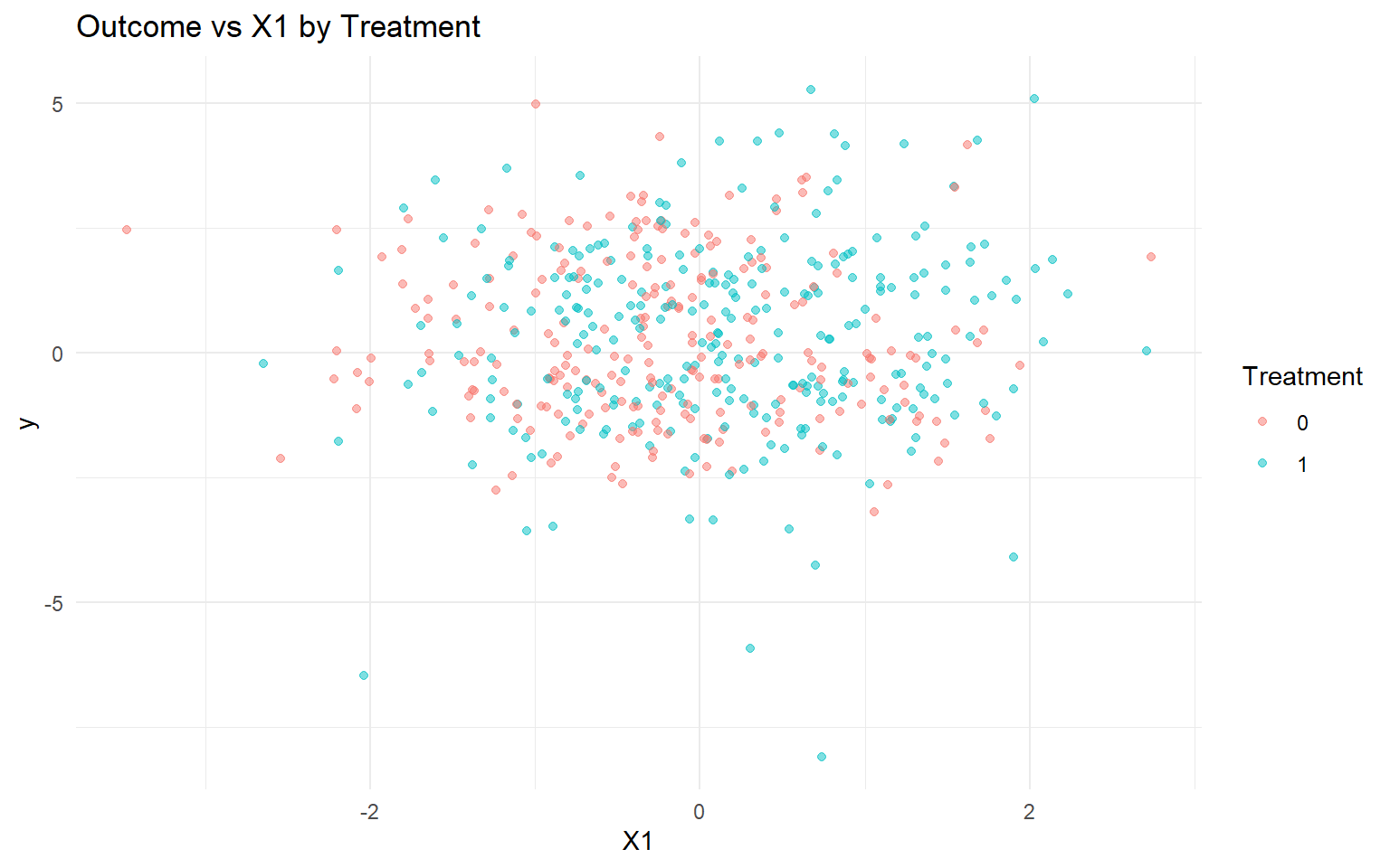
df_causal <- data.frame(y = y, A = as.factor(A), x1 = X[, 1], x2 = X[, 2])

p_scatter <- ggplot(df_causal, aes(x = x1, y = y, color = A)) +
  geom_point(alpha = 0.5) +
  labs(title = "Outcome vs X1 by Treatment", x = "X1", y = "y", color = "Treatment") +
  theme_minimal()

p_scatter

Model A: SB Bulk-only (Laplace)

Code

bundle_sb_bulk <- bundle(
  y = y,
  treat = A,
  X = X,
  kernel = "laplace",
  backend = "sb",
  PS = "logit",
  GPD = FALSE,
  components = components_ex12,
  mcmc_outcome = bulk_mcmc_ex12,
  mcmc_ps = mcmc_ps_bulk_ex12
)

bundle_sb_bulk

CausalMixGPD causal bundle
PS model: Bayesian logit (A | X) 
      Field                Treated                Control
    Backend Stick-Breaking Process Stick-Breaking Process
     Kernel                laplace                laplace
 Components                      3                      3
   GPD tail                  FALSE                  FALSE
    Epsilon                  0.025                  0.025

Outcome PS included: TRUE 
n (control) = 232 | n (treated) = 268

Code

summary(bundle_sb_bulk)

CausalMixGPD causal bundle summary
CausalMixGPD causal bundle
PS model: Bayesian logit (A | X) 
      Field                Treated                Control
    Backend Stick-Breaking Process Stick-Breaking Process
     Kernel                laplace                laplace
 Components                      3                      3
   GPD tail                  FALSE                  FALSE
    Epsilon                  0.025                  0.025

Outcome PS included: TRUE 
n (control) = 232 | n (treated) = 268

Code

fit_sb_bulk <- load_or_fit(
  tag_sb_bulk_ex12,
  quiet_mcmc(dpmix.causal(bundle_sb_bulk, mcmc = causal_run_mcmc_bulk))
)
summary(fit_sb_bulk)

-- PS fit --
CausalMixGPD PS fit summary
model: logit 
n = 500 | predictors = 5
Monitors: beta 

Summary table
 parameter   mean    sd q0.025 q0.500 q0.975
   beta[1]  0.031 0.186 -0.234 -0.009  0.456
   beta[2]  0.463  0.13  0.168  0.524  0.646
   beta[3]   0.41 0.209  0.103  0.461   0.82
   beta[4] -0.185 0.075 -0.281 -0.117 -0.116
   beta[5]  0.235 0.305  -0.42  0.247   0.74

-- Outcome fits --
[control]
MixGPD summary | backend: Stick-Breaking Process | kernel: Laplace Distribution | GPD tail: FALSE | epsilon: 0.025
n = 232 | components = 3
Summary
Initial components: 3 | Components after truncation: 3

Summary table
          parameter  mean    sd q0.025 q0.500 q0.975
         weights[1] 0.377 0.018  0.346   0.37  0.405
         weights[2] 0.332 0.023  0.298  0.328  0.358
         weights[3] 0.291 0.017  0.272   0.29  0.326
              alpha 1.233 0.723  0.491  0.986   3.16
           scale[1] 0.805 0.101  0.648  0.804  1.061
           scale[2] 0.783 0.119  0.596  0.777  1.082
           scale[3] 0.748 0.121  0.521  0.727  1.022
 beta_location[1,1]     0     0      0      0      0
 beta_location[1,2]     0     0      0      0      0
 beta_location[1,3]     0     0      0      0      0
 beta_location[1,4]     0     0      0      0      0
 beta_location[2,1]     0     0      0      0      0
 beta_location[2,2]     0     0      0      0      0
 beta_location[2,3]     0     0      0      0      0
 beta_location[2,4]     0     0      0      0      0
 beta_location[3,1]     0     0      0      0      0
 beta_location[3,2]     0     0      0      0      0
 beta_location[3,3]     0     0      0      0      0
 beta_location[3,4]     0     0      0      0      0

[treated]
MixGPD summary | backend: Stick-Breaking Process | kernel: Laplace Distribution | GPD tail: FALSE | epsilon: 0.025
n = 268 | components = 3
Summary
Initial components: 3 | Components after truncation: 3

Summary table
          parameter  mean    sd q0.025 q0.500 q0.975
         weights[1] 0.698 0.017  0.679  0.713  0.713
         weights[2] 0.161 0.013  0.144  0.162  0.186
         weights[3] 0.141 0.021  0.101  0.143   0.16
              alpha 1.069 0.548   0.25  0.888  2.367
           scale[1] 0.685 0.073  0.568  0.677  0.838
           scale[2] 0.675 0.184  0.469  0.632  1.239
           scale[3] 0.674 0.154  0.433  0.654   1.03
 beta_location[1,1]     0     0      0      0      0
 beta_location[1,2]     0     0      0      0      0
 beta_location[1,3]     0     0      0      0      0
 beta_location[1,4]     0     0      0      0      0
 beta_location[2,1]     0     0      0      0      0
 beta_location[2,2]     0     0      0      0      0
 beta_location[2,3]     0     0      0      0      0
 beta_location[2,4]     0     0      0      0      0
 beta_location[3,1]     0     0      0      0      0
 beta_location[3,2]     0     0      0      0      0
 beta_location[3,3]     0     0      0      0      0
 beta_location[3,4]     0     0      0      0      0

Code

params(fit_sb_bulk)

Posterior mean parameters (causal)

[ps]
Posterior mean parameters

$beta
[1]  0.03087  0.46270  0.40980 -0.18530  0.23550

[treated]
Posterior mean parameters

$alpha
[1] 1.069

$w
[1] 0.6980 0.1607 0.1413

$beta_location
      PropScore x1 x2 x3 x4
comp1         0  0  0  0  0
comp2         0  0  0  0  0
comp3         0  0  0  0  0

$scale
[1] 0.6849 0.6750 0.6736

[control]
Posterior mean parameters

$alpha
[1] 1.233

$w
[1] 0.3765 0.3322 0.2913

$beta_location
      PropScore x1 x2 x3 x4
comp1         0  0  0  0  0
comp2         0  0  0  0  0
comp3         0  0  0  0  0

$scale
[1] 0.8050 0.7825 0.7482

Code

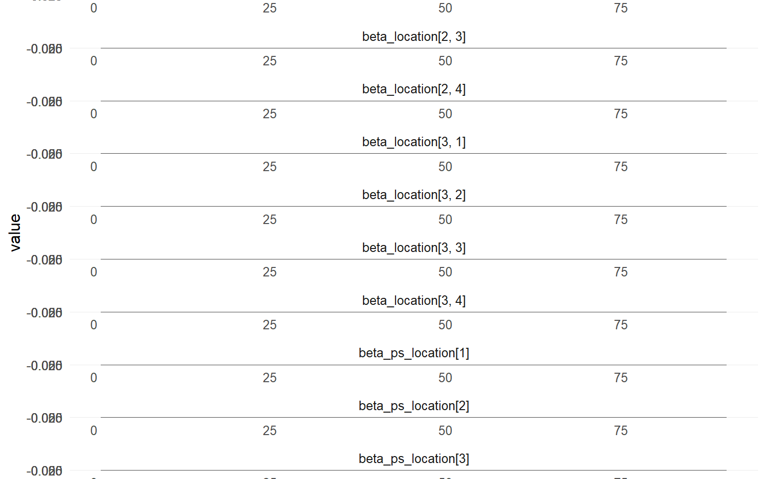
plot(fit_sb_bulk, family = plot_family_bulk_ex12)


=== treated ===

=== traceplot ===


=== control ===

=== traceplot ===

Code

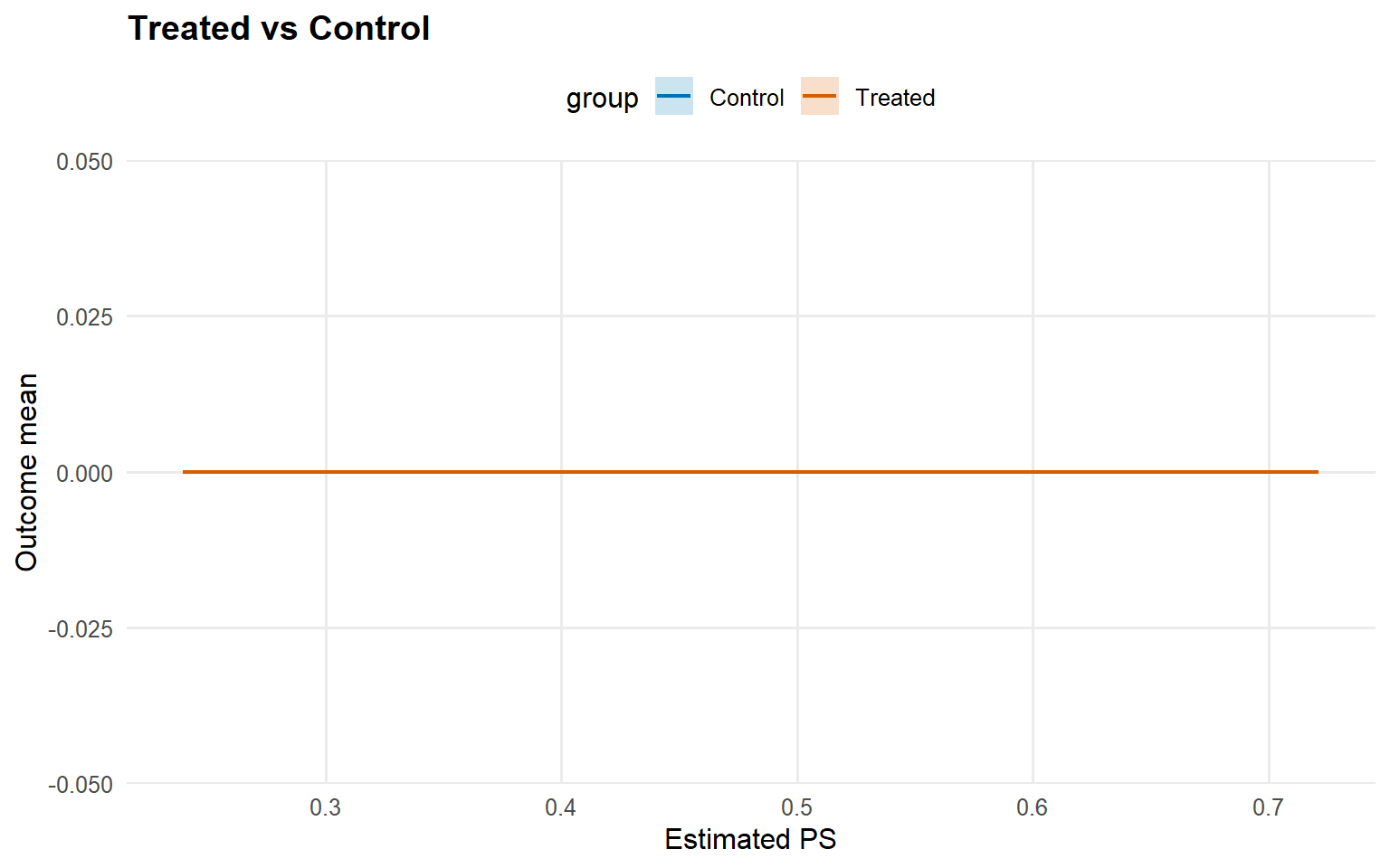
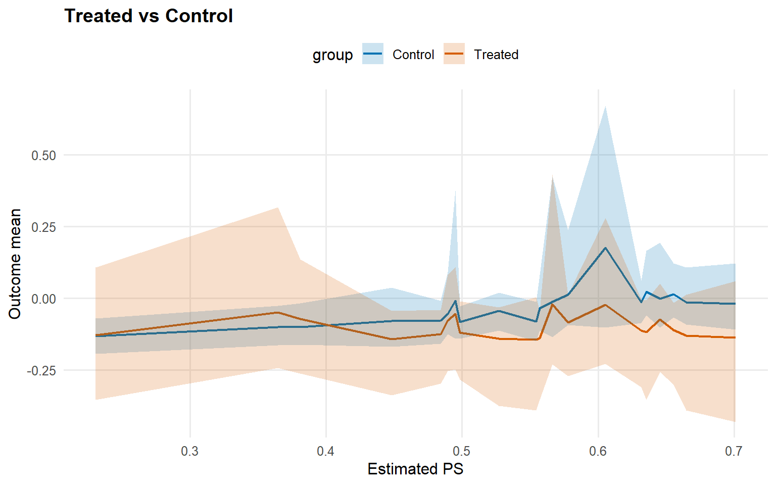
pred_mean_bulk <- predict(fit_sb_bulk, newdata =x_eval, type = "mean",
                          interval = "credible", nsim_mean = nsim_mean_ex12, workers = predict_workers_ex12)
plot(pred_mean_bulk)

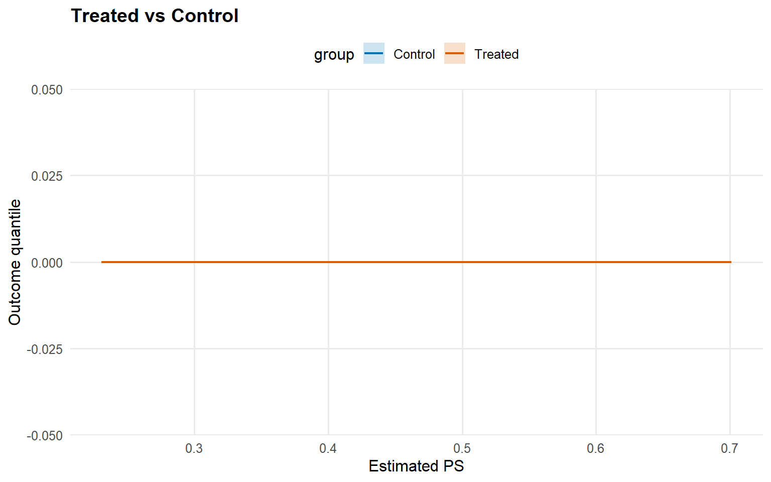
Code

pred_q_bulk <- predict(fit_sb_bulk, newdata =x_eval, type = "quantile",
                       p = 0.5, interval = "credible", workers = predict_workers_ex12)
plot(pred_q_bulk)

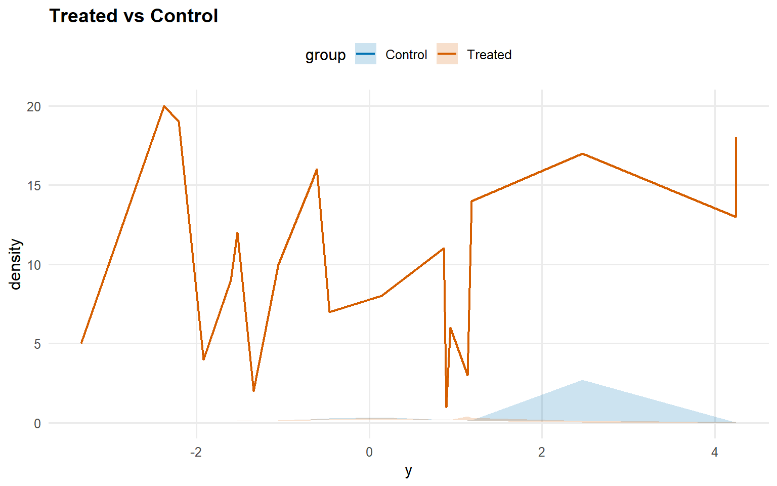
Code

pred_d_bulk <- predict(fit_sb_bulk, newdata =x_eval, y = y_eval,
                       type = "density", interval = "credible", workers = predict_workers_ex12)
plot(pred_d_bulk)

Code

pred_surv_bulk <- predict(fit_sb_bulk, newdata =x_eval, y = y_eval,
                          type = "survival", interval = "credible", workers = predict_workers_ex12)
plot(pred_surv_bulk)

Code

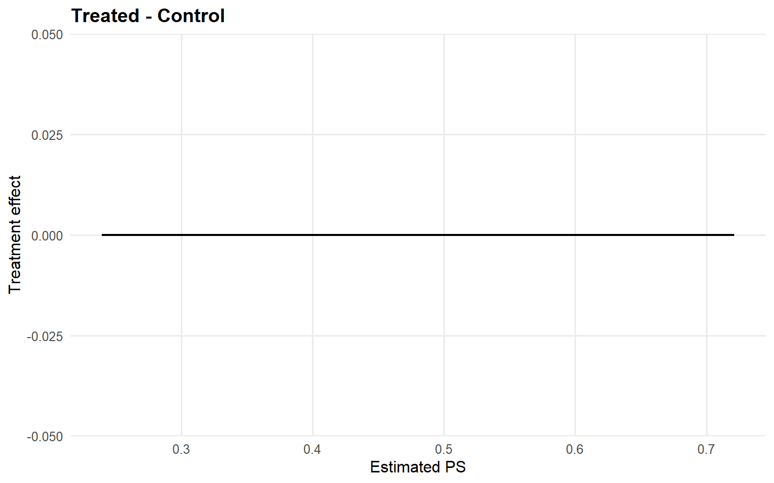
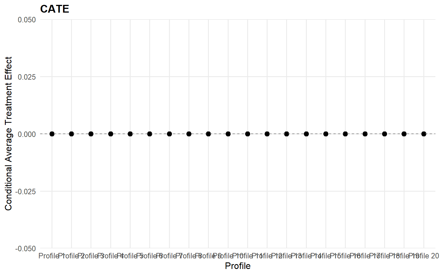
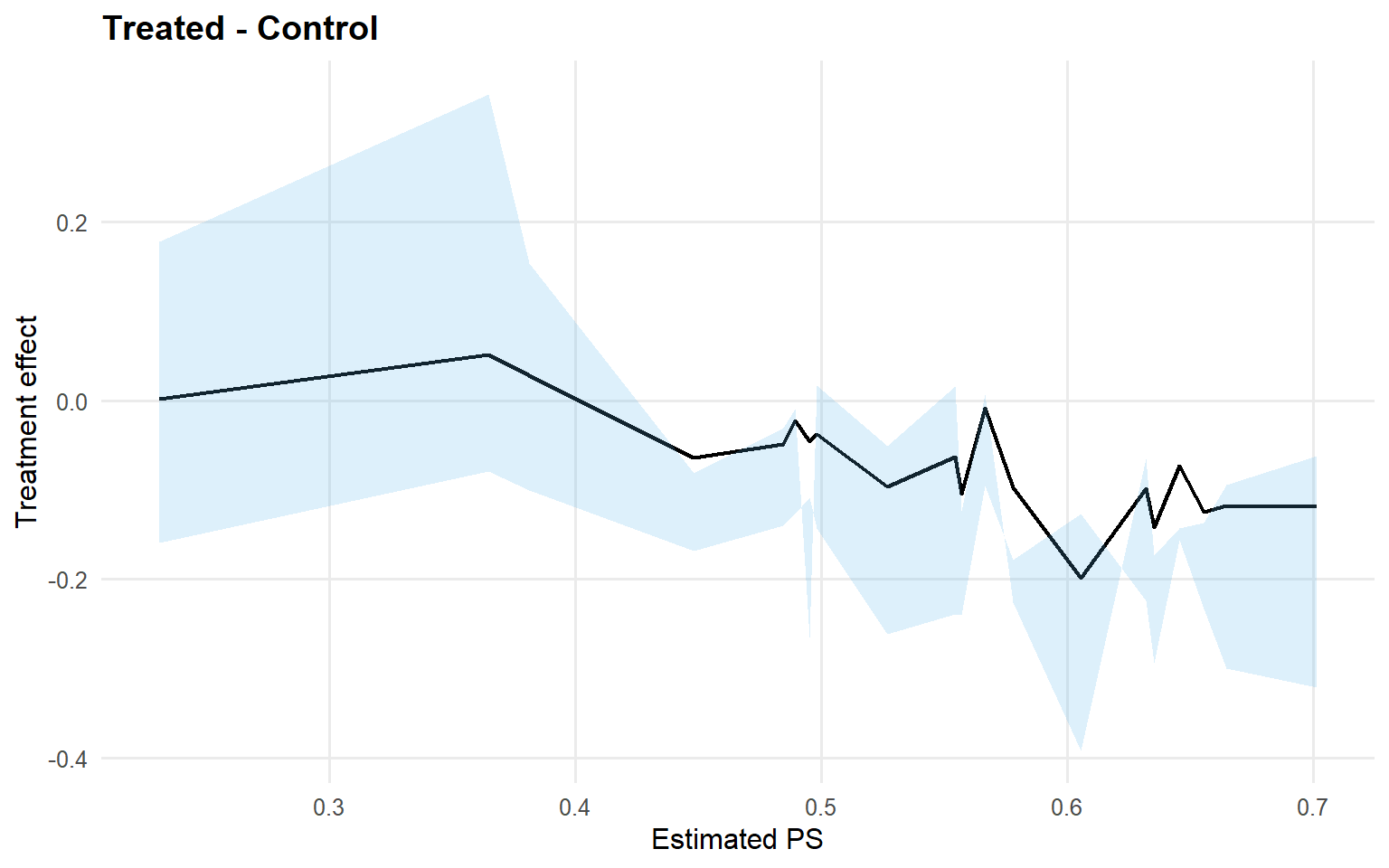
cate_bulk <- cate(fit_sb_bulk, newdata = x_eval,
                 interval = "credible", nsim_mean = nsim_mean_ex12)
head(format_cate_table(cate_bulk))

  id index estimate lower upper
1  1     1        0     0     0
2  2     1        0     0     0
3  3     1        0     0     0
4  4     1        0     0     0
5  5     1        0     0     0
6  6     1        0     0     0

Code

plot(cate_bulk)

Code

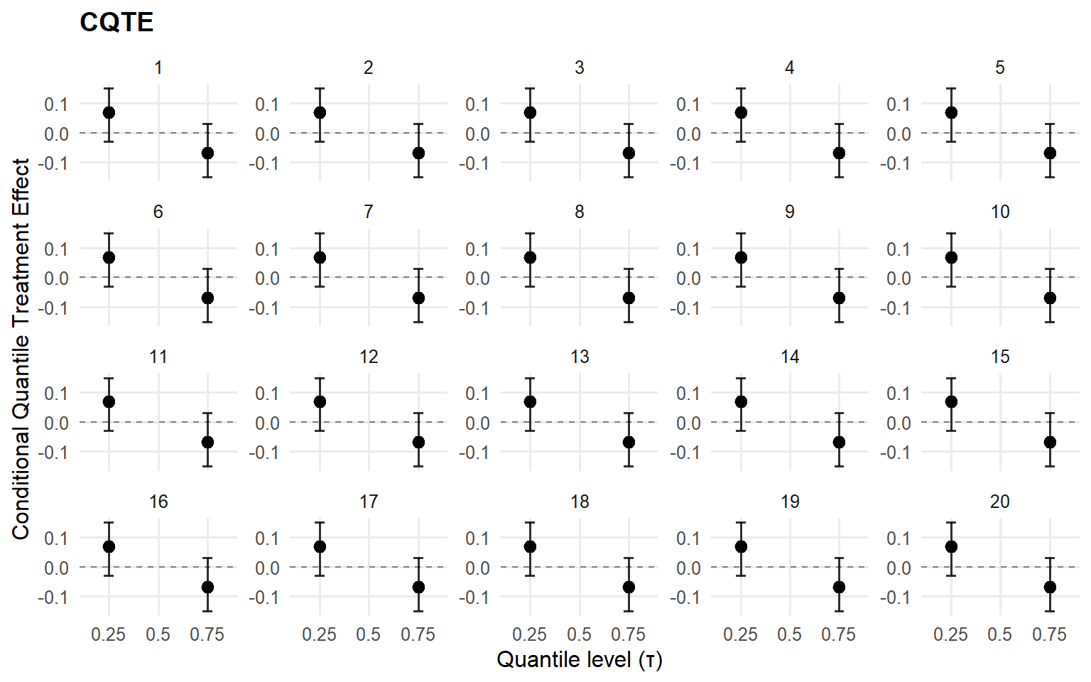
cqte_bulk <- cqte(fit_sb_bulk, probs = c(0.25, 0.5, 0.75),
                 newdata = x_eval, interval = "credible")
head(format_cqte_table(cqte_bulk))

  id index    estimate      lower     upper
1  1     1  0.06878438 -0.0300103 0.1503468
2  1     2         NaN         NA        NA
3  1     3 -0.06878438 -0.1503468 0.0300103
4  2     1  0.06878438 -0.0300103 0.1503468
5  2     2         NaN         NA        NA
6  2     3 -0.06878438 -0.1503468 0.0300103

Code

plot(cqte_bulk)

Model B: SB with GPD Tail (Laplace)

Code

param_specs_gpd <- list(
  gpd = list(
    threshold = list(
      mode = "dist",
      dist = "lognormal",
      args = list(meanlog = log(max(u_threshold, .Machine$double.eps)), sdlog = 0.25)
    )
  )
)

bundle_sb_gpd <- bundle(
  y = y,
  treat = A,
  X = X,
  kernel = "laplace",
  backend = "sb",
  PS = "logit",
  GPD = TRUE,
  components = components_ex12,
  param_specs = param_specs_gpd,
  mcmc_outcome = gpd_mcmc_ex12,
  mcmc_ps = mcmc_ps_gpd_ex12
)

bundle_sb_gpd

CausalMixGPD causal bundle
PS model: Bayesian logit (A | X) 
      Field                Treated                Control
    Backend Stick-Breaking Process Stick-Breaking Process
     Kernel                laplace                laplace
 Components                      3                      3
   GPD tail                   TRUE                   TRUE
    Epsilon                  0.025                  0.025

Outcome PS included: TRUE 
n (control) = 232 | n (treated) = 268

Code

summary(bundle_sb_gpd)

CausalMixGPD causal bundle summary
CausalMixGPD causal bundle
PS model: Bayesian logit (A | X) 
      Field                Treated                Control
    Backend Stick-Breaking Process Stick-Breaking Process
     Kernel                laplace                laplace
 Components                      3                      3
   GPD tail                   TRUE                   TRUE
    Epsilon                  0.025                  0.025

Outcome PS included: TRUE 
n (control) = 232 | n (treated) = 268

Code

fit_sb_gpd <- load_or_fit(
  tag_sb_gpd_ex12,
  quiet_mcmc(dpmgpd.causal(bundle_sb_gpd, mcmc = causal_run_mcmc_gpd))
)
summary(fit_sb_gpd)

-- PS fit --
CausalMixGPD PS fit summary
model: logit 
n = 500 | predictors = 5
Monitors: beta 

Summary table
 parameter   mean    sd q0.025 q0.500 q0.975
   beta[1]  0.021 0.082 -0.056 -0.005  0.144
   beta[2]  0.458 0.082  0.324  0.451  0.607
   beta[3]   0.27 0.197 -0.042  0.216  0.544
   beta[4] -0.149 0.065 -0.303 -0.107  -0.07
   beta[5]  0.277 0.149 -0.228  0.348   0.48

-- Outcome fits --
[control]
MixGPD summary | backend: Stick-Breaking Process | kernel: Laplace Distribution | GPD tail: TRUE | epsilon: 0.025
n = 232 | components = 3
Summary
Initial components: 3 | Components after truncation: 3

Summary table
          parameter   mean    sd q0.025 q0.500 q0.975
         weights[1]  0.665 0.002  0.662  0.666  0.666
         weights[2]  0.281 0.013  0.264  0.288  0.302
         weights[3]  0.054 0.015  0.035  0.046  0.074
              alpha  1.094 0.551  0.475  1.027  2.832
 beta_tail_scale[1]  0.545  0.26  0.116   0.56  0.996
 beta_tail_scale[2]  0.078 0.321 -0.472   0.12  0.648
 beta_tail_scale[3] -0.019 0.262  -0.44 -0.009  0.507
 beta_tail_scale[4] -0.555 0.397 -1.214 -0.589   0.15
         tail_shape  0.182 0.188 -0.286  0.176  0.414
          threshold  2.427 0.088  2.151   2.46   2.46
           scale[1]   1.43  0.15  1.186  1.443  1.719
           scale[2]  1.502 0.247  1.123  1.466  1.958
           scale[3]  1.889 0.989  0.644  1.646  4.361
 beta_location[1,1]      0     0      0      0      0
 beta_location[1,2]      0     0      0      0      0
 beta_location[1,3]      0     0      0      0      0
 beta_location[1,4]      0     0      0      0      0
 beta_location[2,1]      0     0      0      0      0
 beta_location[2,2]      0     0      0      0      0
 beta_location[2,3]      0     0      0      0      0
 beta_location[2,4]      0     0      0      0      0
 beta_location[3,1]      0     0      0      0      0
 beta_location[3,2]      0     0      0      0      0
 beta_location[3,3]      0     0      0      0      0
 beta_location[3,4]      0     0      0      0      0

[treated]
MixGPD summary | backend: Stick-Breaking Process | kernel: Laplace Distribution | GPD tail: TRUE | epsilon: 0.025
n = 268 | components = 3
Summary
Initial components: 3 | Components after truncation: 3

Summary table
          parameter   mean    sd q0.025 q0.500 q0.975
         weights[1]  0.452 0.038  0.437  0.437  0.551
         weights[2]  0.321 0.026  0.285   0.32  0.361
         weights[3]  0.227 0.035  0.161  0.243  0.278
              alpha  1.447 0.968  0.206  1.282  3.431
 beta_tail_scale[1]  0.154 0.256 -0.278  0.118  0.734
 beta_tail_scale[2]  0.063 0.369 -0.463  0.011   0.75
 beta_tail_scale[3]  0.149 0.162 -0.143  0.152  0.478
 beta_tail_scale[4]  0.038 0.536 -0.842 -0.018  1.333
         tail_shape -0.144 0.269 -0.583 -0.209  0.226
          threshold  2.306 1.025  1.069  2.001  4.037
           scale[1]   1.68 0.253  1.339  1.645  2.287
           scale[2]   1.73  0.29  1.242  1.708  2.319
           scale[3]  1.585 0.511  1.062  1.398  3.161
 beta_location[1,1]      0     0      0      0      0
 beta_location[1,2]      0     0      0      0      0
 beta_location[1,3]      0     0      0      0      0
 beta_location[1,4]      0     0      0      0      0
 beta_location[2,1]      0     0      0      0      0
 beta_location[2,2]      0     0      0      0      0
 beta_location[2,3]      0     0      0      0      0
 beta_location[2,4]      0     0      0      0      0
 beta_location[3,1]      0     0      0      0      0
 beta_location[3,2]      0     0      0      0      0
 beta_location[3,3]      0     0      0      0      0
 beta_location[3,4]      0     0      0      0      0

Code

params(fit_sb_gpd)

Posterior mean parameters (causal)

[ps]
Posterior mean parameters

$beta
[1]  0.02086  0.45850  0.27050 -0.14870  0.27740

[treated]
Posterior mean parameters

$alpha
[1] 1.447

$w
[1] 0.4521 0.3205 0.2274

$beta_location
      PropScore x1 x2 x3 x4
comp1         0  0  0  0  0
comp2         0  0  0  0  0
comp3         0  0  0  0  0

$scale
[1] 1.680 1.730 1.585

$threshold
[1] 2.306

$beta_tail_scale
            x1     x2    x3      x4
overall 0.1536 0.0633 0.149 0.03797

$tail_shape
[1] -0.1438

[control]
Posterior mean parameters

$alpha
[1] 1.094

$w
[1] 0.66460 0.28140 0.05398

$beta_location
      PropScore x1 x2 x3 x4
comp1         0  0  0  0  0
comp2         0  0  0  0  0
comp3         0  0  0  0  0

$scale
[1] 1.430 1.502 1.889

$threshold
[1] 2.427

$beta_tail_scale
            x1     x2       x3      x4
overall 0.5454 0.0782 -0.01914 -0.5554

$tail_shape
[1] 0.1823

Code

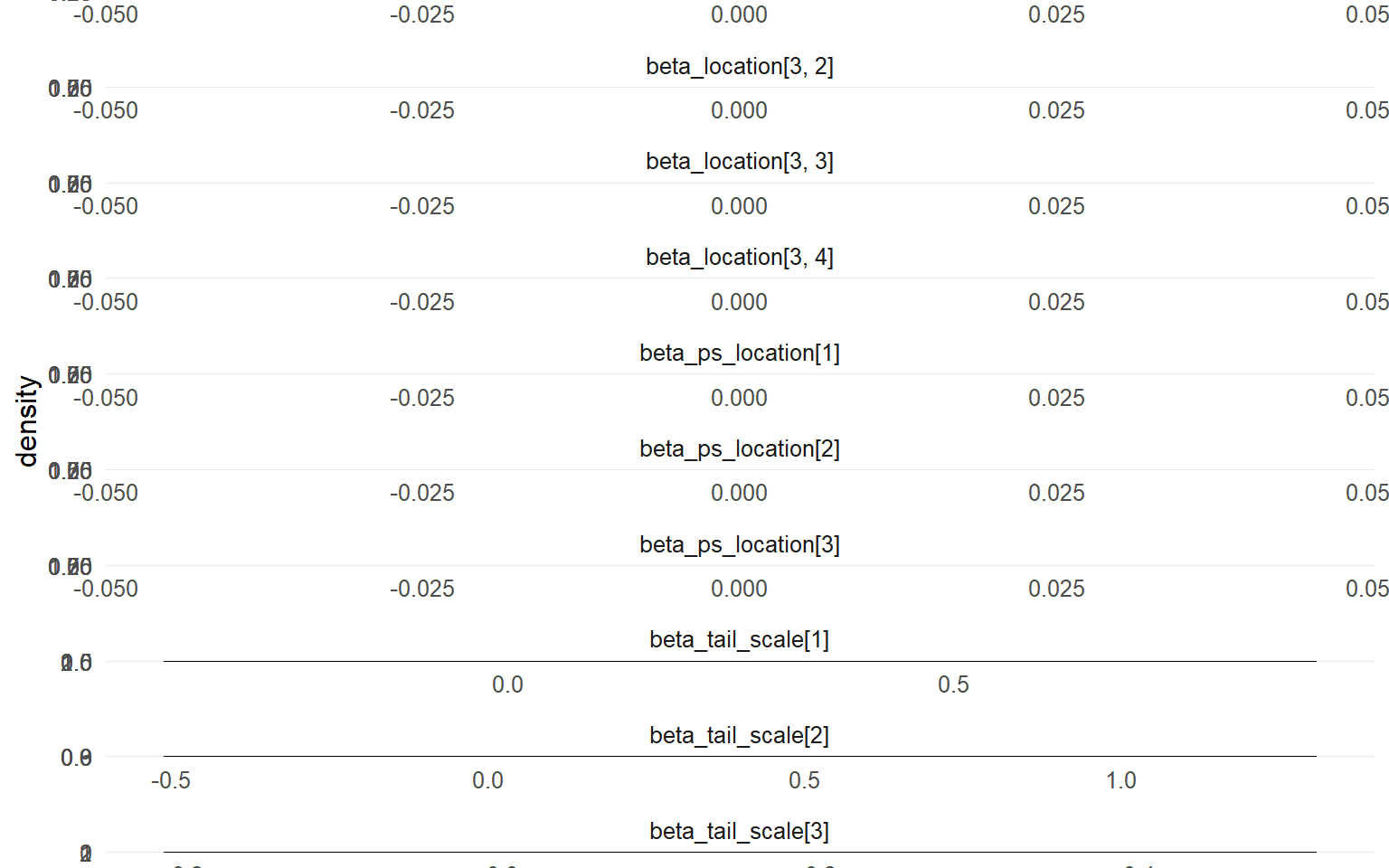
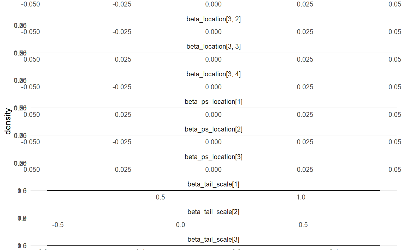
plot(fit_sb_gpd, family = plot_family_gpd_ex12)


=== treated ===

=== density ===


=== control ===

=== density ===

Code

pred_mean_gpd <- predict(fit_sb_gpd, newdata =x_eval, type = "mean",
                         interval = "credible", nsim_mean = nsim_mean_ex12, workers = predict_workers_ex12)
plot(pred_mean_gpd)

Code

pred_q_gpd <- predict(fit_sb_gpd, newdata =x_eval, type = "quantile",
                      p = 0.5, interval = "credible", workers = predict_workers_ex12)
plot(pred_q_gpd)

Code

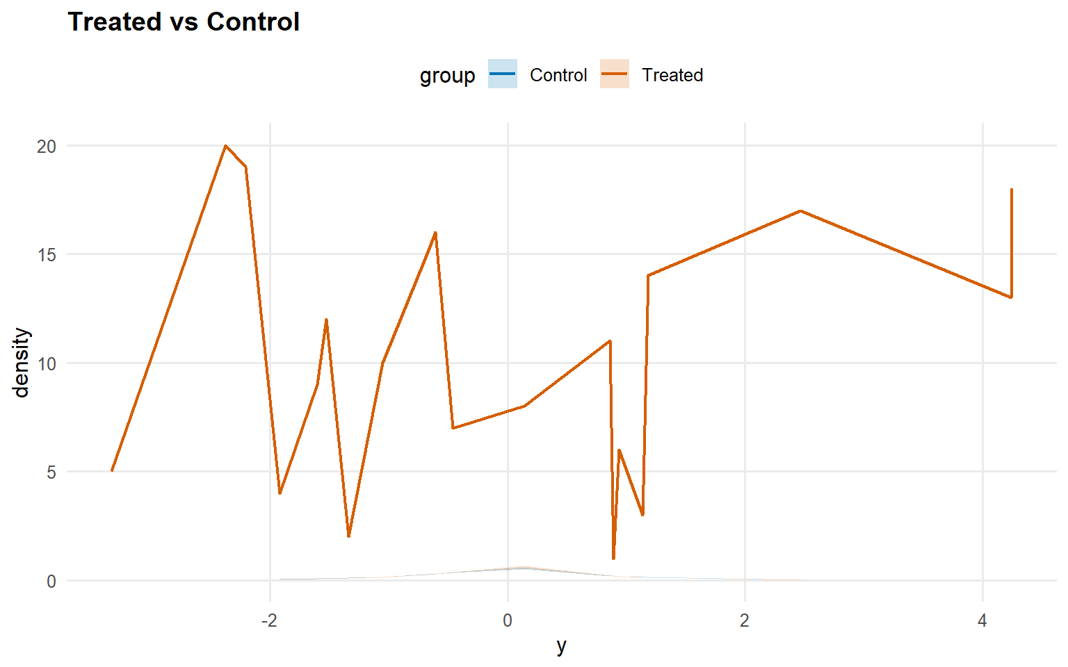
pred_d_gpd <- predict(fit_sb_gpd, newdata =x_eval, y = y_eval,
                      type = "density", interval = "credible", workers = predict_workers_ex12)
plot(pred_d_gpd)

Code

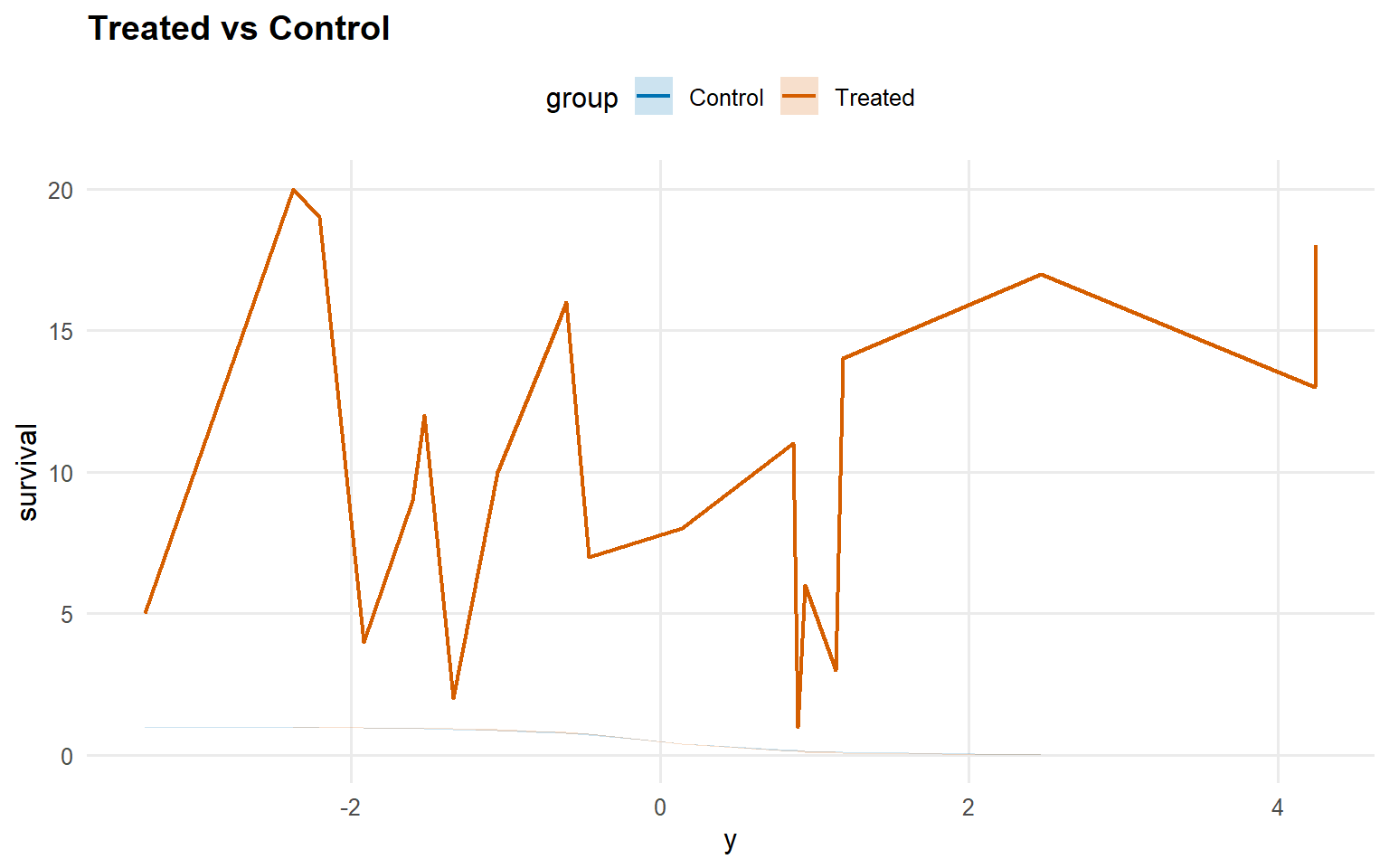
pred_surv_gpd <- predict(fit_sb_gpd, newdata =x_eval, y = y_eval,
                         type = "survival", interval = "credible", workers = predict_workers_ex12)
plot(pred_surv_gpd)

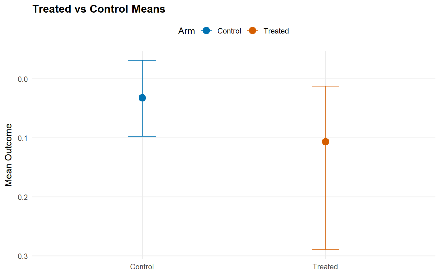
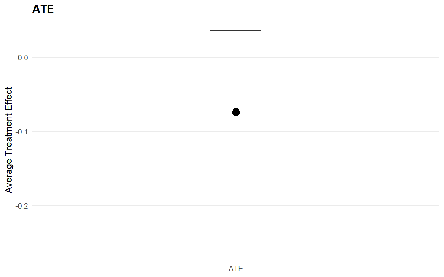
Code

ate_gpd <- ate(fit_sb_gpd, interval = "credible", nsim_mean = nsim_mean_ex12)
plot(ate_gpd)

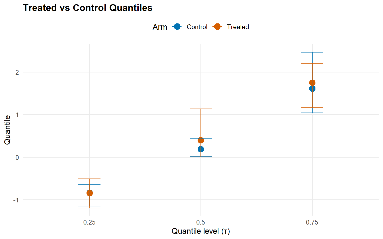
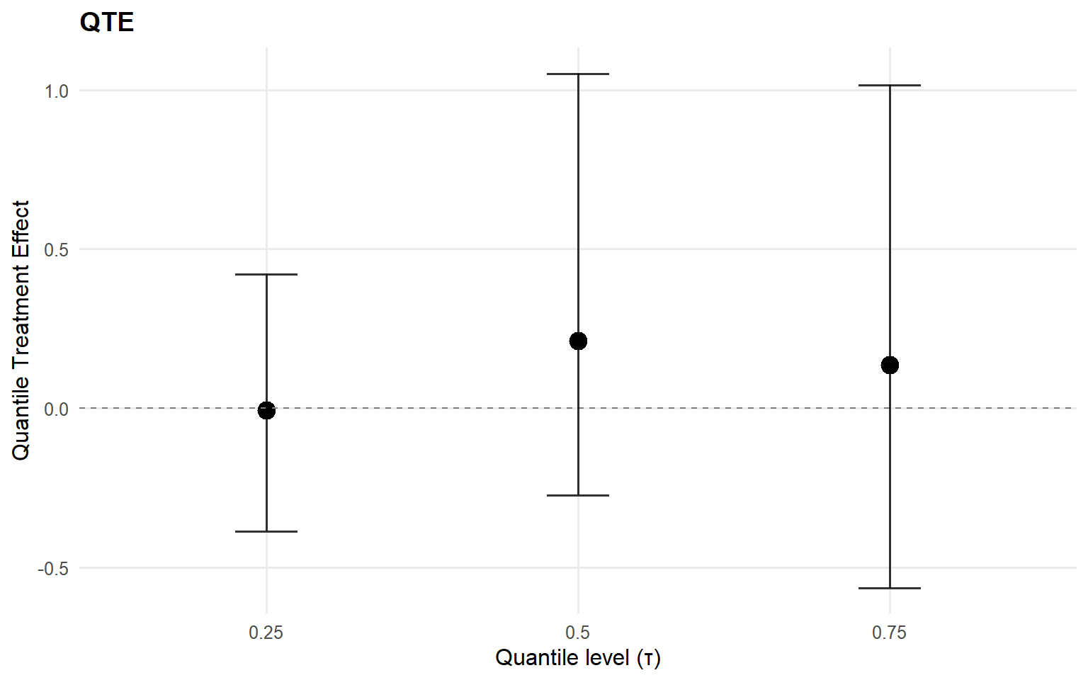
Code

qte_gpd <- qte(fit_sb_gpd, probs = c(0.25, 0.5, 0.75), interval = "credible")
plot(qte_gpd)

Prereqs

Required packages and data for this page are listed in the setup chunks above.

Outputs

This page renders model fits, diagnostics, and summary artifacts generated by package APIs.

Interpretation

Canonical concept page: 03 Causal Inference Objects
Treat this page as an application/example view and use the canonical page for core definitions.

Continue to the linked canonical concept page, then return for implementation-specific details.

ex12. Causal (Same backend, SB Backend) - Laplace Kernel

Causal Inference: Same Backend (SB) - Laplace Kernel

What you’ll learn

When to use this template

Data Setup

Model A: SB Bulk-only (Laplace)

Model B: SB with GPD Tail (Laplace)

Workflow Navigation

Prereqs

Outputs

Interpretation

Next