ex13. Causal (Different backends, CRP Backend) - Cauchy Kernel

Website workflow note. This page reflects the current exported API and recommended wrapper-first usage. Last updated: 2026-02-19.

For the full package narrative, see the main package vignettes (basic, unconditional, conditional, and causal).

Causal Inference: Mixed Backends (Bulk-only) - Cauchy Kernel

This vignette fits two mixed-backend causal models with a shared Cauchy kernel:

Model A: Treated = SB, Control = CRP
Model B: Treated = CRP, Control = SB

What you’ll learn

How to specify arm-specific backends (treated vs control) within one causal bundle.
How to interpret causal predictions/effects when the two potential-outcome models have different partition structures.
How to keep the comparison focused on backend differences by using a shared kernel and GPD = FALSE.

When to use this template

You suspect treated and control outcomes differ in ways that make one backend preferable for one arm.
You want to study how much causal estimands change under backend asymmetry while keeping tail modeling off.

Next steps

Turn on tail augmentation (mixed-backend + GPD = TRUE) when extremes plausibly drive effect heterogeneity.
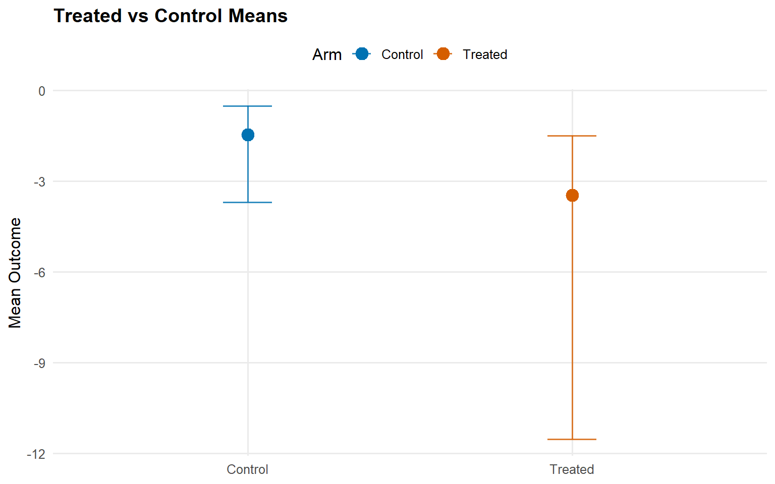
Because the Cauchy kernel does not have a finite mean, this page uses median and upper-quantile predictions, plus restricted-mean causal effects.

Data Setup

Code

data("causal_alt_real500_p4_k2")
y <- causal_alt_real500_p4_k2$y
A <- causal_alt_real500_p4_k2$A
X <- as.matrix(causal_alt_real500_p4_k2$X)

summary_tbl <- tibble(
  statistic = c("N", "Mean", "SD", "Min", "Max"),
  value = c(length(y), mean(y), sd(y), min(y), max(y))
)

summary_tbl

# A tibble: 5 × 2
  statistic   value
  <chr>       <dbl>
1 N         500    
2 Mean        0.274
3 SD          1.76 
4 Min        -8.09 
5 Max         5.27

Code

x_eval <- X[seq_len(if (isTRUE(FAST)) 20L else 40L), , drop = FALSE]
y_eval <- y[seq_len(if (isTRUE(FAST)) 20L else 40L)]

Code

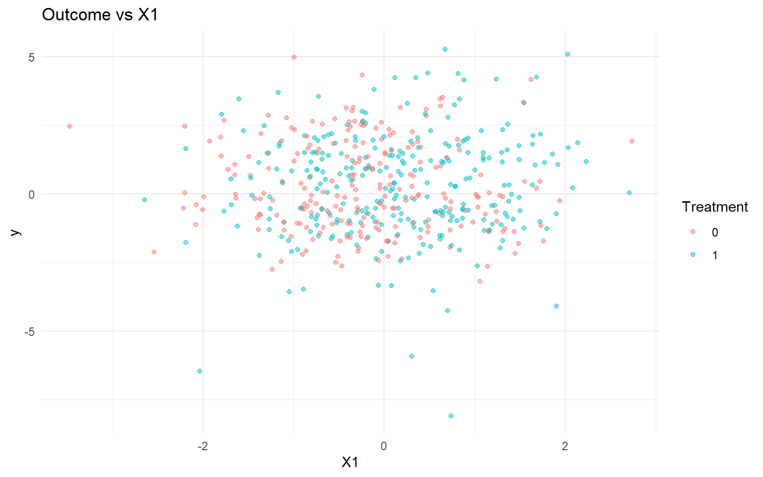
df_causal <- data.frame(y = y, A = as.factor(A), x1 = X[, 1])

p_scatter <- ggplot(df_causal, aes(x = x1, y = y, color = A)) +
  geom_point(alpha = 0.5) +
  labs(title = "Outcome vs X1", x = "X1", y = "y", color = "Treatment") +
  theme_minimal()

p_scatter

Model A: Treated SB, Control CRP (Cauchy)

Code

bundle_sb_crp <- bundle(
  y = y,
  treat = A,
  X = X,
  kernel = c("cauchy", "cauchy"),
  backend = c("sb", "crp"),
  PS = "logit",
  GPD = c(FALSE, FALSE),
  components = components_ex13,
  mcmc_outcome = bulk_mcmc_ex13,
  mcmc_ps = mcmc_ps_ex13
)

bundle_sb_crp

CausalMixGPD causal bundle
PS model: Bayesian logit (A | X) 
      Field                Treated                    Control
    Backend Stick-Breaking Process Chinese Restaurant Process
     Kernel                 cauchy                     cauchy
 Components                      3                          3
   GPD tail                  FALSE                      FALSE
    Epsilon                  0.025                      0.025

Outcome PS included: TRUE 
n (control) = 232 | n (treated) = 268

Code

summary(bundle_sb_crp)

CausalMixGPD causal bundle summary
CausalMixGPD causal bundle
PS model: Bayesian logit (A | X) 
      Field                Treated                    Control
    Backend Stick-Breaking Process Chinese Restaurant Process
     Kernel                 cauchy                     cauchy
 Components                      3                          3
   GPD tail                  FALSE                      FALSE
    Epsilon                  0.025                      0.025

Outcome PS included: TRUE 
n (control) = 232 | n (treated) = 268

Code

fit_sb_crp <- load_or_fit(
  tag_sb_crp_ex13,
  quiet_mcmc(dpmix.causal(bundle_sb_crp, mcmc = causal_run_mcmc))
)
summary(fit_sb_crp)

-- PS fit --
CausalMixGPD PS fit summary
model: logit 
n = 500 | predictors = 5
Monitors: beta 

Summary table
 parameter   mean    sd q0.025 q0.500 q0.975
   beta[1]  0.031 0.186 -0.234 -0.009  0.456
   beta[2]  0.463  0.13  0.168  0.524  0.646
   beta[3]   0.41 0.209  0.103  0.461   0.82
   beta[4] -0.185 0.075 -0.281 -0.117 -0.116
   beta[5]  0.235 0.305  -0.42  0.247   0.74

-- Outcome fits --
[control]
MixGPD summary | backend: Chinese Restaurant Process | kernel: Cauchy Distribution | GPD tail: FALSE | epsilon: 0.025
n = 232 | components = 3
Summary
Initial components: 3 | Components after truncation: 3

WAIC: 942.038
lppd: -361.955 | pWAIC: 109.064

Summary table
          parameter   mean    sd q0.025 q0.500 q0.975
         weights[1]  0.453 0.063  0.358  0.455  0.599
         weights[2]   0.36 0.036  0.297  0.358  0.427
         weights[3]  0.187 0.071  0.066  0.183  0.306
              alpha  0.449 0.306  0.103  0.368  1.077
           scale[1]  0.701 0.149  0.466  0.697  1.046
           scale[2]  0.647 0.152  0.382  0.653  0.986
           scale[3]  0.622 0.173  0.339  0.626  0.978
 beta_location[1,1]  -0.27 0.557 -1.096 -0.037   0.39
 beta_location[1,2]  0.119 0.347 -0.529  0.119  0.703
 beta_location[1,3] -0.242 0.232 -0.688 -0.208   0.02
 beta_location[1,4]  0.732 1.441 -0.916 -0.146  2.485
 beta_location[2,1] -0.321 0.458 -0.934 -0.375  0.341
 beta_location[2,2] -0.071 0.462 -0.873 -0.067  0.713
 beta_location[2,3] -0.177 0.214 -0.551 -0.113  0.058
 beta_location[2,4]  0.669 1.532  -1.44  1.824  2.329
 beta_location[3,1]  0.258 0.309 -0.366  0.289    0.7
 beta_location[3,2] -0.478 0.467 -1.265 -0.559  0.713
 beta_location[3,3]  0.069  0.32 -0.522  0.058  0.773
 beta_location[3,4] -0.584 0.678 -1.429 -0.885  1.572

[treated]
MixGPD summary | backend: Stick-Breaking Process | kernel: Cauchy Distribution | GPD tail: FALSE | epsilon: 0.025
n = 268 | components = 3
Summary
Initial components: 3 | Components after truncation: 3

Summary table
          parameter  mean    sd q0.025 q0.500 q0.975
         weights[1] 0.664 0.043  0.593   0.66  0.741
         weights[2] 0.201 0.033  0.154  0.203   0.27
         weights[3] 0.135 0.025  0.088  0.136  0.182
              alpha 1.272 0.641  0.129  1.147   2.63
           scale[1]  1.16 0.109  0.971  1.162  1.343
           scale[2] 1.199 0.251   0.74   1.19  1.699
           scale[3] 1.311  0.38  0.747  1.232  2.277
 beta_location[1,1]     0     0      0      0      0
 beta_location[1,2]     0     0      0      0      0
 beta_location[1,3]     0     0      0      0      0
 beta_location[1,4]     0     0      0      0      0
 beta_location[2,1]     0     0      0      0      0
 beta_location[2,2]     0     0      0      0      0
 beta_location[2,3]     0     0      0      0      0
 beta_location[2,4]     0     0      0      0      0
 beta_location[3,1]     0     0      0      0      0
 beta_location[3,2]     0     0      0      0      0
 beta_location[3,3]     0     0      0      0      0
 beta_location[3,4]     0     0      0      0      0

Code

params(fit_sb_crp)

Posterior mean parameters (causal)

[ps]
Posterior mean parameters

$beta
[1]  0.03087  0.46270  0.40980 -0.18530  0.23550

[treated]
Posterior mean parameters

$alpha
[1] 1.272

$w
[1] 0.6642 0.2008 0.1350

$beta_location
      PropScore x1 x2 x3 x4
comp1         0  0  0  0  0
comp2         0  0  0  0  0
comp3         0  0  0  0  0

$scale
[1] 1.160 1.199 1.311

[control]
Posterior mean parameters

$alpha
[1] 0.4488

$w
[1] 0.4528 0.3599 0.1873

$beta_location
      PropScore      x1       x2       x3      x4
comp1    0.1207 -0.2704  0.11890 -0.24190  0.7316
comp2    0.1856 -0.3205 -0.07111 -0.17740  0.6692
comp3   -0.9230  0.2583 -0.47790  0.06883 -0.5837

$scale
[1] 0.7009 0.6470 0.6218

Code

plot(fit_sb_crp, family = plot_family_sb_crp_ex13)


=== treated ===

=== traceplot ===


=== control ===

=== traceplot ===

Code

pred_median_sb_crp <- predict(
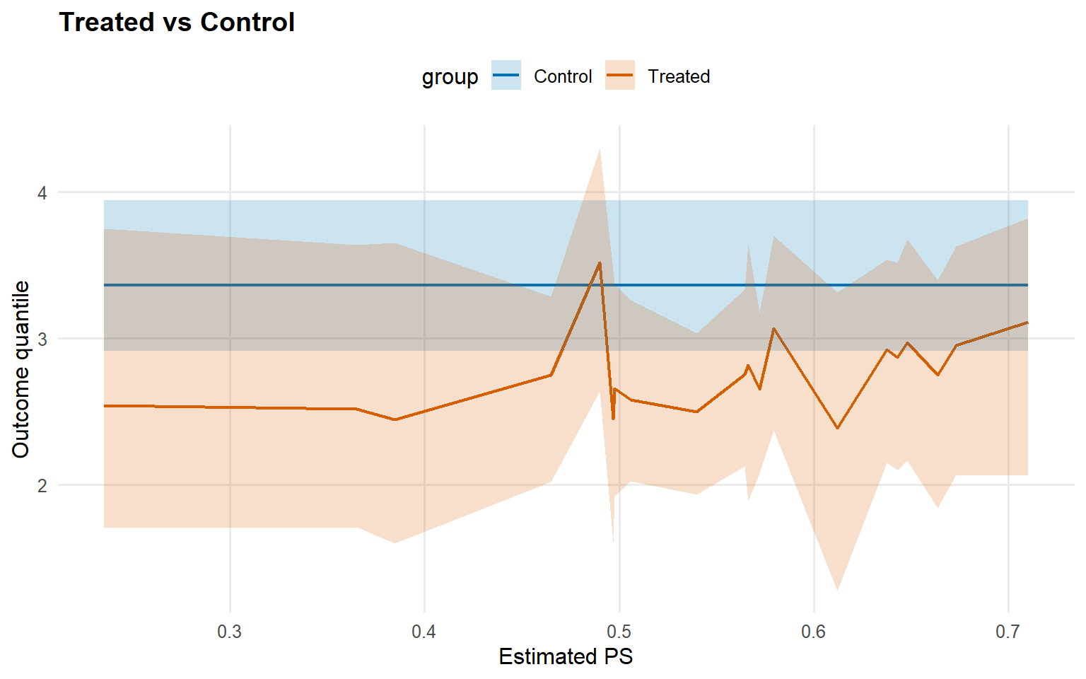
  fit_sb_crp,
  newdata =x_eval,
  type = "quantile",
  p = 0.5,
  interval = "credible",
  workers = predict_workers_ex13
)
plot(pred_median_sb_crp)

Code

pred_q_sb_crp <- predict(fit_sb_crp, newdata =x_eval, type = "quantile",
                         p = 0.9, interval = "credible", workers = predict_workers_ex13)
plot(pred_q_sb_crp)

Code

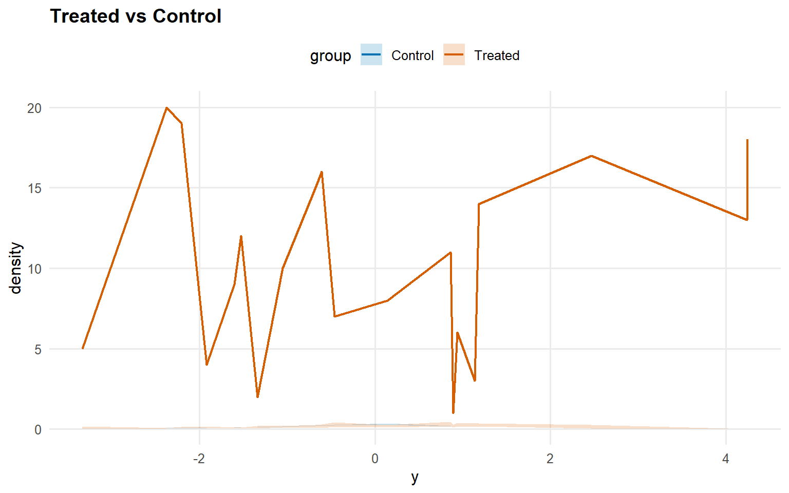
pred_d_sb_crp <- predict(fit_sb_crp, newdata =x_eval, y = y_eval,
                         type = "density", interval = "credible", workers = predict_workers_ex13)
plot(pred_d_sb_crp)

Code

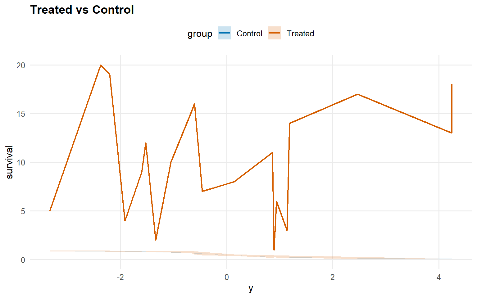
pred_surv_sb_crp <- predict(fit_sb_crp, newdata =x_eval, y = y_eval,
                            type = "survival", interval = "credible", workers = predict_workers_ex13)
plot(pred_surv_sb_crp)

Code

att_sb_crp <- att(
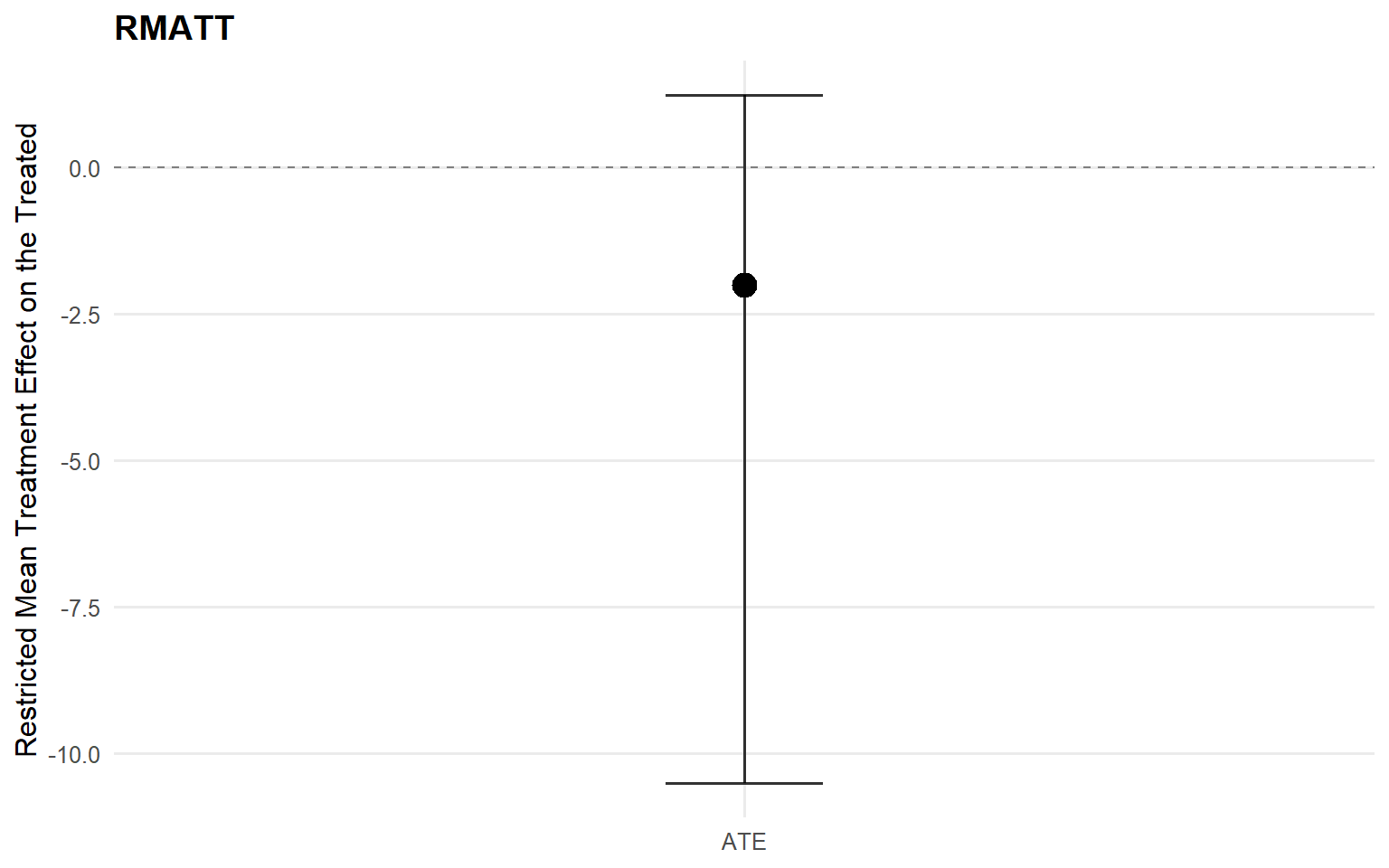
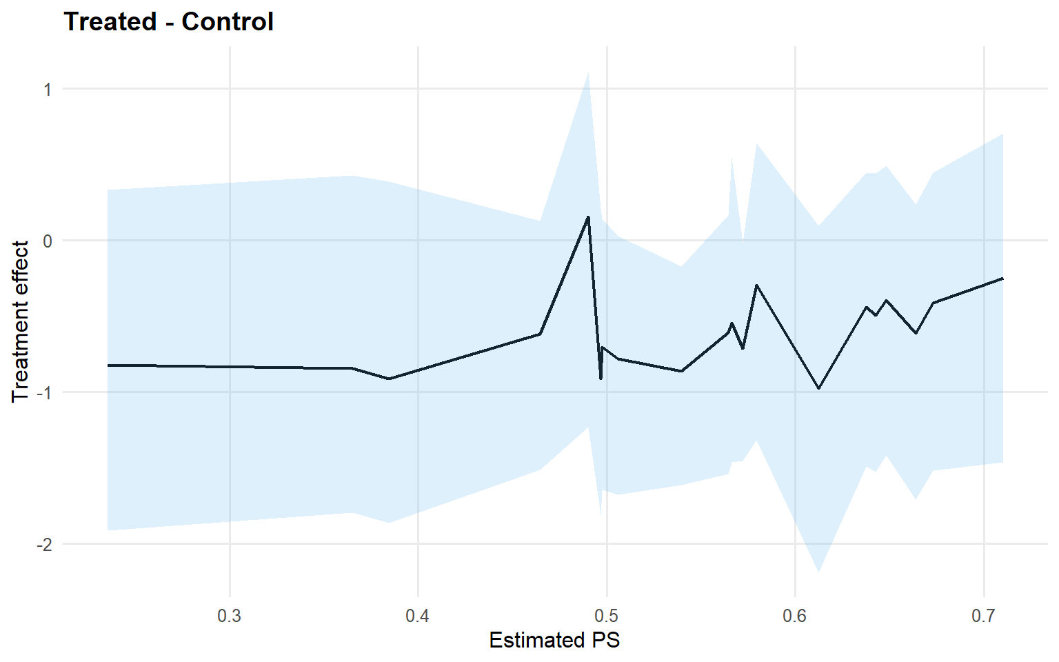
  fit_sb_crp,
  type = "rmean",
  cutoff = rmean_cutoff_ex13,
  interval = "credible",
  nsim_mean = nsim_mean_ex13
)
plot(att_sb_crp)

Code

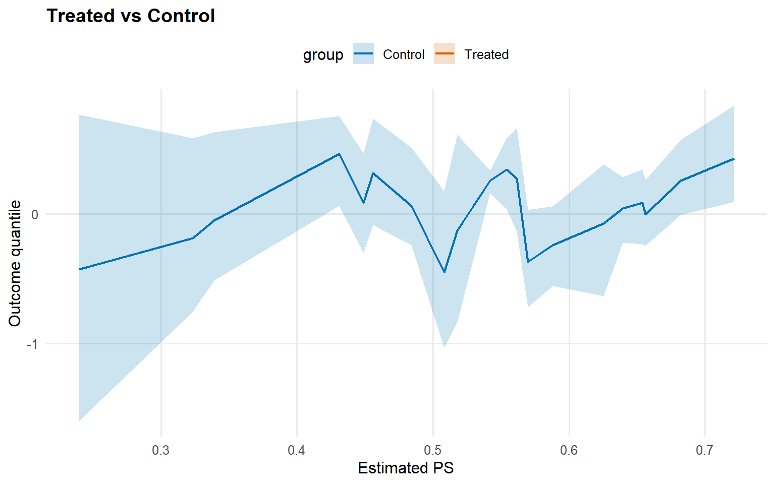
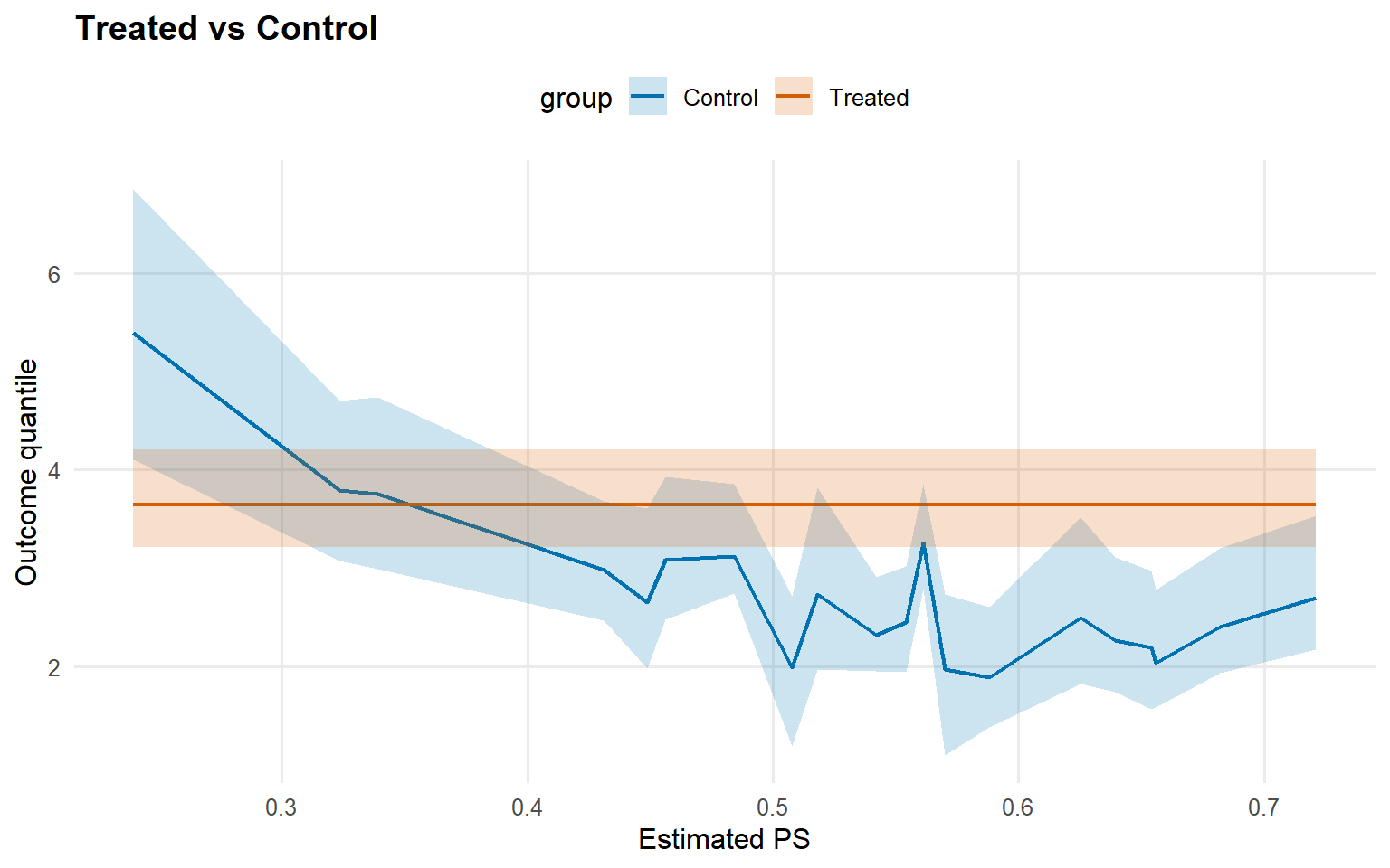
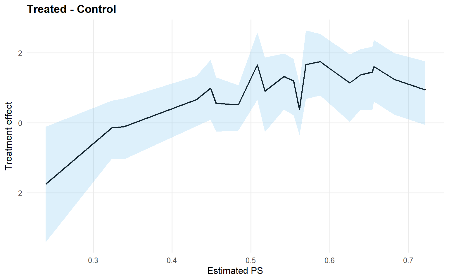
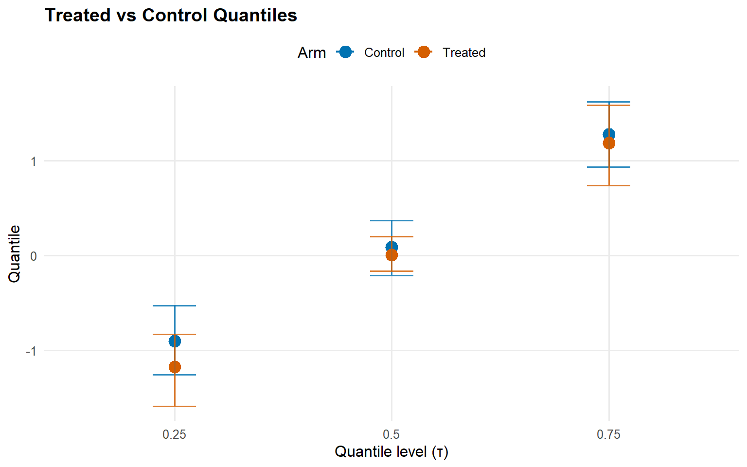
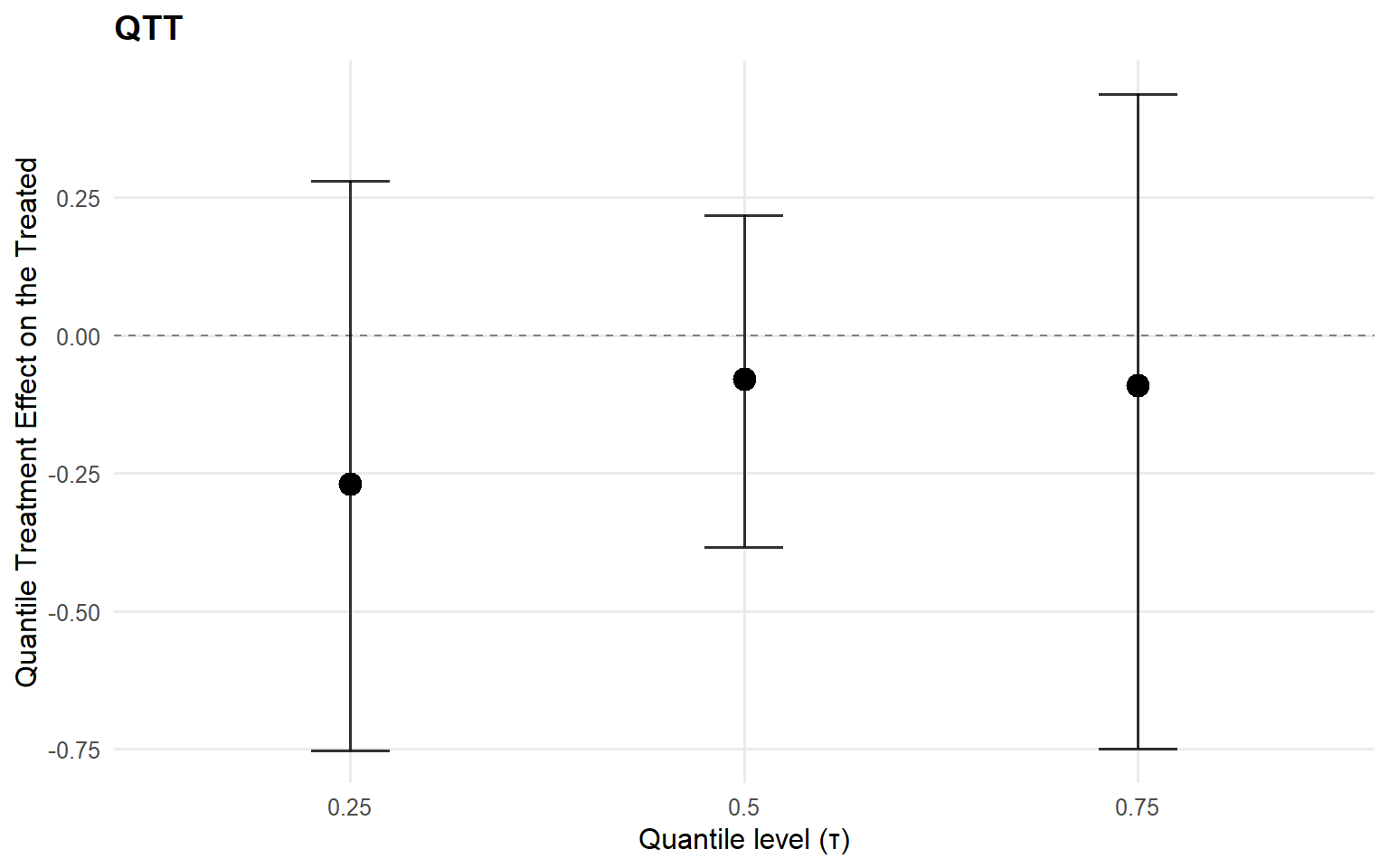
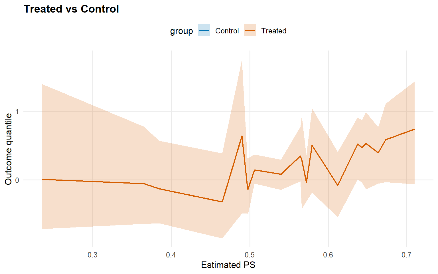
qtt_sb_crp <- qtt(fit_sb_crp, probs = c(0.25, 0.5, 0.75), interval = "credible")
plot(qtt_sb_crp)

Model B: Treated CRP, Control SB (Cauchy)

Code

bundle_crp_sb <- bundle(
  y = y,
  treat = A,
  X = X,
  kernel = c("cauchy", "cauchy"),
  backend = c("crp", "sb"),
  PS = "logit",
  GPD = c(FALSE, FALSE),
  components = components_ex13,
  mcmc_outcome = bulk_mcmc_ex13_b,
  mcmc_ps = mcmc_ps_ex13_b
)

bundle_crp_sb

CausalMixGPD causal bundle
PS model: Bayesian logit (A | X) 
      Field                    Treated                Control
    Backend Chinese Restaurant Process Stick-Breaking Process
     Kernel                     cauchy                 cauchy
 Components                          3                      3
   GPD tail                      FALSE                  FALSE
    Epsilon                      0.025                  0.025

Outcome PS included: TRUE 
n (control) = 232 | n (treated) = 268

Code

summary(bundle_crp_sb)

CausalMixGPD causal bundle summary
CausalMixGPD causal bundle
PS model: Bayesian logit (A | X) 
      Field                    Treated                Control
    Backend Chinese Restaurant Process Stick-Breaking Process
     Kernel                     cauchy                 cauchy
 Components                          3                      3
   GPD tail                      FALSE                  FALSE
    Epsilon                      0.025                  0.025

Outcome PS included: TRUE 
n (control) = 232 | n (treated) = 268

Code

fit_crp_sb <- load_or_fit(
  tag_crp_sb_ex13,
  quiet_mcmc(dpmix.causal(bundle_crp_sb, mcmc = causal_run_mcmc))
)
summary(fit_crp_sb)

-- PS fit --
CausalMixGPD PS fit summary
model: logit 
n = 500 | predictors = 5
Monitors: beta 

Summary table
 parameter   mean    sd q0.025 q0.500 q0.975
   beta[1]  0.059 0.092 -0.056  0.067  0.264
   beta[2]  0.458 0.116  0.215  0.456  0.586
   beta[3]  0.258 0.166  0.041    0.2  0.544
   beta[4] -0.167 0.093 -0.315 -0.128 -0.028
   beta[5]   0.26 0.156 -0.142  0.348  0.458

-- Outcome fits --
[control]
MixGPD summary | backend: Stick-Breaking Process | kernel: Cauchy Distribution | GPD tail: FALSE | epsilon: 0.025
n = 232 | components = 3
Summary
Initial components: 3 | Components after truncation: 3

Summary table
          parameter  mean    sd q0.025 q0.500 q0.975
         weights[1]  0.76 0.006  0.747  0.762  0.767
         weights[2] 0.166 0.016   0.14  0.174  0.185
         weights[3] 0.073 0.018  0.053  0.061  0.098
              alpha 0.731 0.343  0.152  0.683  1.473
           scale[1] 1.078 0.109   0.87  1.093  1.245
           scale[2] 1.187 0.413   0.57  1.176  2.408
           scale[3] 1.098 0.471  0.526  1.024  2.012
 beta_location[1,1]     0     0      0      0      0
 beta_location[1,2]     0     0      0      0      0
 beta_location[1,3]     0     0      0      0      0
 beta_location[1,4]     0     0      0      0      0
 beta_location[2,1]     0     0      0      0      0
 beta_location[2,2]     0     0      0      0      0
 beta_location[2,3]     0     0      0      0      0
 beta_location[2,4]     0     0      0      0      0
 beta_location[3,1]     0     0      0      0      0
 beta_location[3,2]     0     0      0      0      0
 beta_location[3,3]     0     0      0      0      0
 beta_location[3,4]     0     0      0      0      0

[treated]
MixGPD summary | backend: Chinese Restaurant Process | kernel: Cauchy Distribution | GPD tail: FALSE | epsilon: 0.025
n = 268 | components = 3
Summary
Initial components: 3 | Components after truncation: 2

WAIC: 1160.258
lppd: -448.99 | pWAIC: 131.139

Summary table
          parameter  mean    sd q0.025 q0.500 q0.975
         weights[1] 0.515 0.064  0.415  0.513  0.637
         weights[2] 0.397 0.058  0.255  0.403  0.481
              alpha 0.427  0.33   0.07   0.35  1.496
           scale[1] 0.826 0.168  0.541  0.821  1.125
           scale[2]  0.69 0.169  0.448  0.647  1.134
 beta_location[1,1] 0.118 0.241 -0.309  0.123  0.523
 beta_location[1,2] 0.345 0.885 -0.912  0.135   1.71
 beta_location[1,3] 0.002 0.439 -0.739    0.1  0.648
 beta_location[1,4] 0.525 0.497 -0.418  0.667  1.177
 beta_location[2,1] 0.235 0.324 -0.348  0.229  0.713
 beta_location[2,2] 0.348 0.975 -1.214  0.042  1.668
 beta_location[2,3] -0.14 0.468 -0.739    0.1  0.398
 beta_location[2,4] 0.313 0.516  -0.41  0.369  1.195

Code

params(fit_crp_sb)

Posterior mean parameters (causal)

[ps]
Posterior mean parameters

$beta
[1]  0.05896  0.45800  0.25750 -0.16720  0.26020

[treated]
Posterior mean parameters

$alpha
[1] 0.427

$w
[1] 0.5148 0.3970

$beta_location
      PropScore     x1     x2        x3     x4
comp1   -0.3378 0.1177 0.3445  0.001586 0.5255
comp2   -0.3749 0.2346 0.3484 -0.140100 0.3132

$scale
[1] 0.8260 0.6899

[control]
Posterior mean parameters

$alpha
[1] 0.7308

$w
[1] 0.76030 0.16640 0.07332

$beta_location
      PropScore x1 x2 x3 x4
comp1         0  0  0  0  0
comp2         0  0  0  0  0
comp3         0  0  0  0  0

$scale
[1] 1.078 1.187 1.098

Code

plot(fit_crp_sb, family = plot_family_crp_sb_ex13)


=== treated ===

=== density ===


=== control ===

=== density ===

Code

pred_median_crp_sb <- predict(
  fit_crp_sb,
  newdata =x_eval,
  type = "quantile",
  p = 0.5,
  interval = "credible",
  workers = predict_workers_ex13
)
plot(pred_median_crp_sb)

Code

pred_q_crp_sb <- predict(fit_crp_sb, newdata =x_eval, type = "quantile",
                         p = 0.9, interval = "credible", workers = predict_workers_ex13)
plot(pred_q_crp_sb)

Code

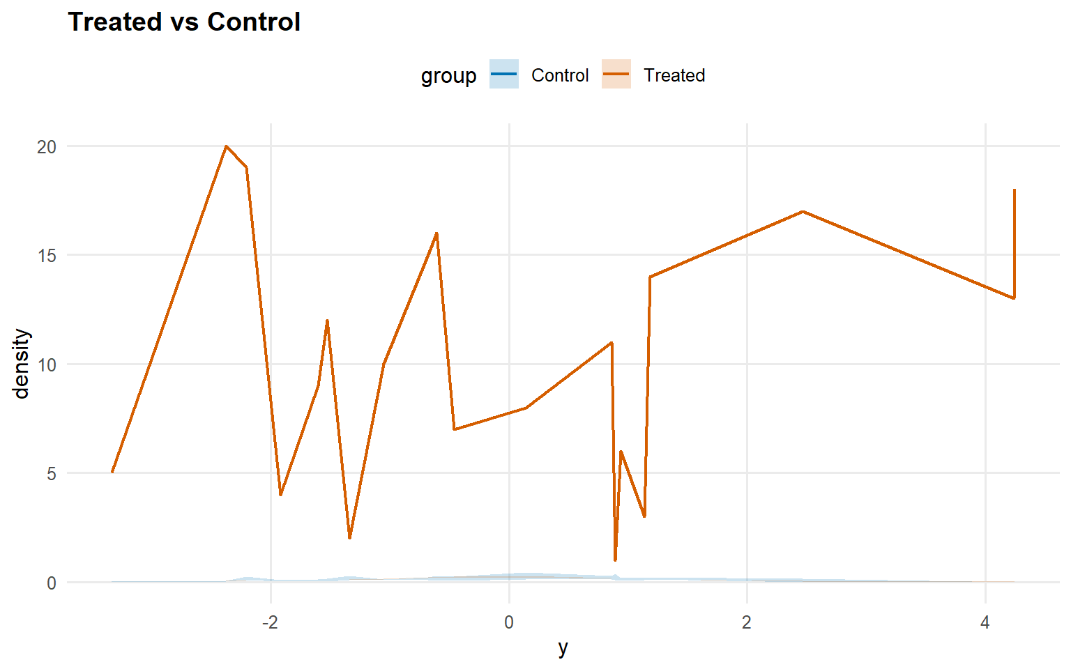
pred_d_crp_sb <- predict(fit_crp_sb, newdata =x_eval, y = y_eval,
                         type = "density", interval = "credible", workers = predict_workers_ex13)
plot(pred_d_crp_sb)

Code

pred_surv_crp_sb <- predict(fit_crp_sb, newdata =x_eval, y = y_eval,
                            type = "survival", interval = "credible", workers = predict_workers_ex13)
plot(pred_surv_crp_sb)

Code

cate_crp_sb <- cate(
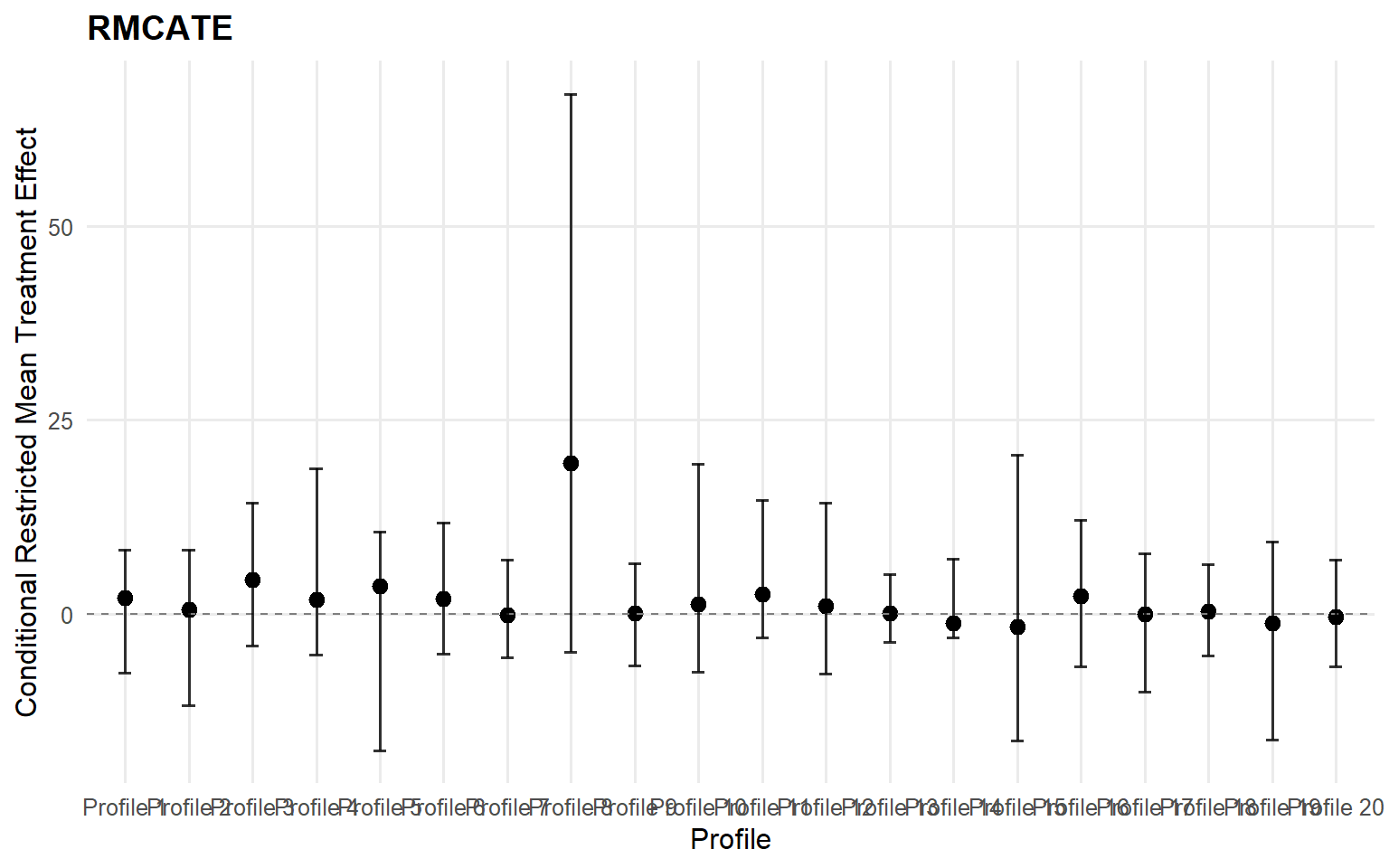
  fit_crp_sb,
  type = "rmean",
  cutoff = rmean_cutoff_ex13,
  newdata = x_eval,
  interval = "credible",
  nsim_mean = nsim_mean_ex13
)
head(format_cate_table(cate_crp_sb))

  id index  estimate      lower     upper
1  1     1 2.0712056  -7.601197  8.232255
2  2     1 0.5246956 -11.766421  8.257291
3  3     1 4.3585056  -4.097305 14.317757
4  4     1 1.8263269  -5.285917 18.786957
5  5     1 3.5740492 -17.630042 10.558621
6  6     1 1.9830236  -5.209355 11.786967

Code

plot(cate_crp_sb)

Code

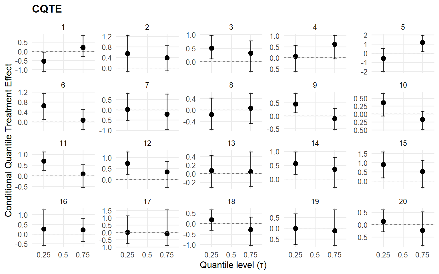
cqte_crp_sb <- cqte(fit_crp_sb, probs = c(0.25, 0.5, 0.75),
                   newdata = x_eval, interval = "credible")
head(format_cqte_table(cqte_crp_sb))

  id index   estimate      lower       upper
1  1     1 -0.5323511 -1.0682313 -0.04068125
2  1     2        NaN         NA          NA
3  1     3  0.2101863 -0.2865770  0.85255201
4  2     1  0.5353392 -0.1215984  1.22619823
5  2     2        NaN         NA          NA
6  2     3  0.3822083 -0.1154588  0.83868138

Code

plot(cqte_crp_sb)

Prereqs

Required packages and data for this page are listed in the setup chunks above.

Outputs

This page renders model fits, diagnostics, and summary artifacts generated by package APIs.

Interpretation

Canonical concept page: 03 Causal Inference Objects
Treat this page as an application/example view and use the canonical page for core definitions.

Continue to the linked canonical concept page, then return for implementation-specific details.

Causal Inference: Mixed Backends (Bulk-only) - Cauchy Kernel

What you’ll learn

When to use this template

Next steps

Because the Cauchy kernel does not have a finite mean, this page uses median and upper-quantile predictions, plus restricted-mean causal effects.

Data Setup

Model A: Treated SB, Control CRP (Cauchy)

Model B: Treated CRP, Control SB (Cauchy)

Workflow Navigation

Prereqs

Outputs

Interpretation

Next