ex14. Causal (Different backends, SB Backend) - Amoroso Kernel

Website workflow note. This page reflects the current exported API and recommended wrapper-first usage. Last updated: 2026-02-19.

For the full package narrative, see the main package vignettes (basic, unconditional, conditional, and causal).

Causal Inference: Mixed Backends with GPD - Amoroso Kernel

This vignette fits two mixed-backend causal models with GPD tails and an Amoroso kernel:

Model A: Treated = SB, Control = CRP
Model B: Treated = CRP, Control = SB

We shift y to keep outcomes in a stable positive range.

What you’ll learn

How to fit mixed-backend causal models when outcomes are shifted positive and modeled with Amoroso bulk + GPD tails.
How tail augmentation influences survival/quantile predictions and downstream effect summaries.
How to keep model comparisons interpretable by reusing the same causal S3 workflow. ## When to use this template
Outcomes are (or can be made) positive and you need a bulk family like Amoroso plus an explicit extreme-tail model.
You want a stress-test style causal analysis where extremes matter and may differ by treatment arm. ## Key limitation (important)

Shifting outcomes changes the scale: interpret effects on the shifted scale (or transform back carefully if you need original-scale statements). ## Next steps

Compare against the bulk-only mixed-backend setup to isolate the incremental impact of GPD = TRUE.

Data Setup

Code

data("causal_alt_real500_p4_k2")
y_raw <- causal_alt_real500_p4_k2$y
A <- causal_alt_real500_p4_k2$A
X <- as.matrix(causal_alt_real500_p4_k2$X)

shift <- abs(min(y_raw)) + 0.1
y <- y_raw + shift

summary_tbl <- tibble(
  statistic = c("N", "Mean", "SD", "Min", "Max"),
  value = c(length(y), mean(y), sd(y), min(y), max(y))
)

summary_tbl

# A tibble: 5 × 2
  statistic    value
  <chr>        <dbl>
1 N         500     
2 Mean        8.46  
3 SD          1.76  
4 Min         0.1000
5 Max        13.5

Code

x_eval <- X[seq_len(if (isTRUE(FAST)) 20L else 40L), , drop = FALSE]
y_eval <- y[seq_len(if (isTRUE(FAST)) 20L else 40L)]
u_threshold <- as.numeric(stats::quantile(y, 0.8, names = FALSE))

Code

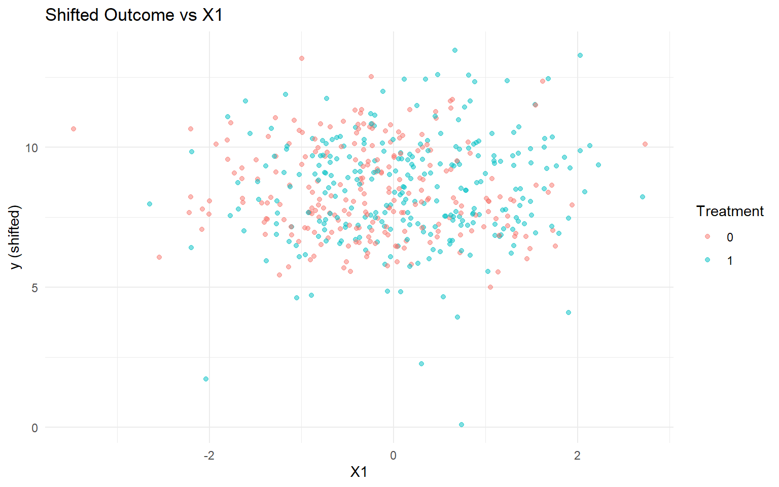
df_causal <- data.frame(y = y, A = as.factor(A), x1 = X[, 1])

p_scatter <- ggplot(df_causal, aes(x = x1, y = y, color = A)) +
  geom_point(alpha = 0.5) +
  labs(title = "Shifted Outcome vs X1", x = "X1", y = "y (shifted)", color = "Treatment") +
  theme_minimal()

p_scatter

Model A: Treated SB, Control CRP (Amoroso + GPD)

Code

param_specs_gpd <- list(
  gpd = list(
    threshold = list(
      mode = "dist",
      dist = "lognormal",
      # Use max() to guard against log(0) = -Inf by enforcing a positive lower bound.
      args = list(meanlog = log(max(u_threshold, .Machine$double.eps)), sdlog = 0.25)
    )
  )
)

bundle_sb_crp <- bundle(
  y = y,
  treat = A,
  X = X,
  kernel = c("amoroso", "amoroso"),
  backend = c("sb", "crp"),
  PS = "logit",
  GPD = c(TRUE, TRUE),
  components = components_ex14,
  param_specs = param_specs_gpd,
  mcmc_outcome = gpd_mcmc_ex14,
  mcmc_ps = mcmc_ps_ex14
)

bundle_sb_crp

CausalMixGPD causal bundle
PS model: Bayesian logit (A | X) 
      Field                Treated                    Control
    Backend Stick-Breaking Process Chinese Restaurant Process
     Kernel                amoroso                    amoroso
 Components                      3                          3
   GPD tail                   TRUE                       TRUE
    Epsilon                  0.025                      0.025

Outcome PS included: TRUE 
n (control) = 232 | n (treated) = 268

Code

summary(bundle_sb_crp)

CausalMixGPD causal bundle summary
CausalMixGPD causal bundle
PS model: Bayesian logit (A | X) 
      Field                Treated                    Control
    Backend Stick-Breaking Process Chinese Restaurant Process
     Kernel                amoroso                    amoroso
 Components                      3                          3
   GPD tail                   TRUE                       TRUE
    Epsilon                  0.025                      0.025

Outcome PS included: TRUE 
n (control) = 232 | n (treated) = 268

Code

fit_sb_crp <- load_or_fit(
  tag_sb_crp_ex14,
  quiet_mcmc(dpmgpd.causal(bundle_sb_crp, mcmc = causal_run_mcmc))
)
summary(fit_sb_crp)

-- PS fit --
CausalMixGPD PS fit summary
model: logit 
n = 500 | predictors = 5
Monitors: beta 

Summary table
 parameter  mean    sd q0.025 q0.500 q0.975
   beta[1]  0.11  0.25 -0.271 -0.091  0.456
   beta[2] 0.474   0.1  0.253  0.509  0.576
   beta[3] 0.394 0.186  0.135  0.395  0.656
   beta[4] -0.15 0.048 -0.277 -0.117 -0.117
   beta[5] 0.101 0.365  -0.42  0.134   0.74

-- Outcome fits --
[control]
MixGPD summary | backend: Chinese Restaurant Process | kernel: Amoroso Distribution | GPD tail: TRUE | epsilon: 0.025
n = 232 | components = 3
Summary
Initial components: 3 | Components after truncation: 1

WAIC: 995.699
lppd: -485.221 | pWAIC: 12.629

Summary table
          parameter   mean    sd q0.025 q0.500 q0.975
         weights[1]      1     0      1      1      1
              alpha  0.192 0.186  0.008  0.123  0.712
 beta_tail_scale[1]  0.089 0.082 -0.055  0.074  0.265
 beta_tail_scale[2]  0.059 0.119 -0.216  0.066  0.272
 beta_tail_scale[3]  0.023 0.087 -0.145  0.032  0.159
 beta_tail_scale[4]  0.365 0.159  0.084  0.376  0.681
         tail_shape -0.234 0.047  -0.28 -0.242 -0.081
          threshold  9.492 0.014  9.454  9.488  9.504
          shape1[1]    5.2 0.283  4.814  5.245  5.585
          shape2[1]  0.705 0.005  0.705  0.705  0.705
      beta_loc[1,1] -0.943  0.16 -1.328 -0.943 -0.721
      beta_loc[1,2]  0.119 0.389 -0.708  0.213  0.559
      beta_loc[1,3]  1.118 0.164  0.719  1.146  1.323
      beta_loc[1,4]  4.761 1.003  2.042  5.202  5.328
    beta_scale[1,1] -0.146 0.168 -0.421 -0.159  0.126
    beta_scale[1,2] -0.278 0.117 -0.489 -0.269 -0.081
    beta_scale[1,3] -0.221 0.083 -0.331 -0.246  0.002
    beta_scale[1,4] -1.082  0.28 -1.437 -1.158 -0.398

[treated]
MixGPD summary | backend: Stick-Breaking Process | kernel: Amoroso Distribution | GPD tail: TRUE | epsilon: 0.025
n = 268 | components = 3
Summary
Initial components: 3 | Components after truncation: 2

Summary table
          parameter   mean    sd q0.025 q0.500 q0.975
         weights[1]  0.783 0.016  0.759  0.774  0.799
         weights[2]   0.17 0.012  0.156  0.167  0.201
              alpha  1.004 0.566  0.253  1.022  2.199
 beta_tail_scale[1]  0.039 0.061 -0.097  0.049  0.153
 beta_tail_scale[2] -0.011 0.097 -0.165  -0.02  0.172
 beta_tail_scale[3]  0.048 0.076  -0.09  0.041  0.193
 beta_tail_scale[4]  1.061  0.12  0.837   1.06   1.24
         tail_shape  -0.02 0.019 -0.046 -0.028   0.01
          threshold  7.173 0.105  6.827  7.204  7.204
          shape1[1]  7.602 0.411  6.985  7.536  8.316
          shape1[2]  5.569 1.256  2.787  5.513  7.623
          shape2[1]  0.888 0.007  0.871   0.89   0.89
          shape2[2]   0.27  0.12  0.112  0.289  0.452
      beta_loc[1,1]      0     0      0      0      0
      beta_loc[1,2]      0     0      0      0      0
      beta_loc[1,3]      0     0      0      0      0
      beta_loc[1,4]      0     0      0      0      0
      beta_loc[2,1]      0     0      0      0      0
      beta_loc[2,2]      0     0      0      0      0
      beta_loc[2,3]      0     0      0      0      0
      beta_loc[2,4]      0     0      0      0      0
    beta_scale[1,1] -0.303 0.122 -0.518 -0.299 -0.095
    beta_scale[1,2] -0.303 0.099 -0.468  -0.31  -0.09
    beta_scale[1,3]   0.13 0.064  0.025  0.133  0.243
    beta_scale[1,4]  -0.13 0.133 -0.367  -0.14  0.089
    beta_scale[2,1]  0.706 1.551 -1.923  0.563   3.96
    beta_scale[2,2]  0.037 1.654 -3.141  0.081  3.161
    beta_scale[2,3] -0.626 1.069 -2.831 -0.828  1.321
    beta_scale[2,4]   1.32 2.616 -3.322  1.316  6.291

Code

params(fit_sb_crp)

Posterior mean parameters (causal)

[ps]
Posterior mean parameters

$beta
[1]  0.1103  0.4739  0.3935 -0.1501  0.1015

[treated]
Posterior mean parameters

$alpha
[1] 1.004

$w
[1] 0.7825 0.1704

$beta_loc
      PropScore x1 x2 x3 x4
comp1         0  0  0  0  0
comp2         0  0  0  0  0

$beta_scale
      PropScore      x1       x2      x3      x4
comp1  0.730200 -0.3029 -0.30320  0.1301 -0.1296
comp2  0.002732  0.7057  0.03679 -0.6260  1.3200

$shape1
[1] 7.602 5.569

$shape2
[1] 0.8878 0.2705

$threshold
[1] 7.173

$beta_tail_scale
             x1       x2      x3    x4
overall 0.03919 -0.01077 0.04789 1.061

$tail_shape
[1] -0.02018

[control]
Posterior mean parameters

$alpha
[1] 0.1923

$w
[1] 1

$beta_loc
      PropScore      x1     x2    x3    x4
comp1     2.473 -0.9426 0.1194 1.118 4.761

$beta_scale
      PropScore      x1     x2      x3     x4
comp1   0.08794 -0.1462 -0.278 -0.2206 -1.082

$shape1
[1] 5.2

$shape2
[1] 0.7054

$threshold
[1] 9.492

$beta_tail_scale
             x1      x2    x3     x4
overall 0.08891 0.05928 0.023 0.3646

$tail_shape
[1] -0.2335

Code

plot(fit_sb_crp, family = plot_family_sb_crp_ex14)


=== treated ===

=== traceplot ===


=== control ===

=== traceplot ===

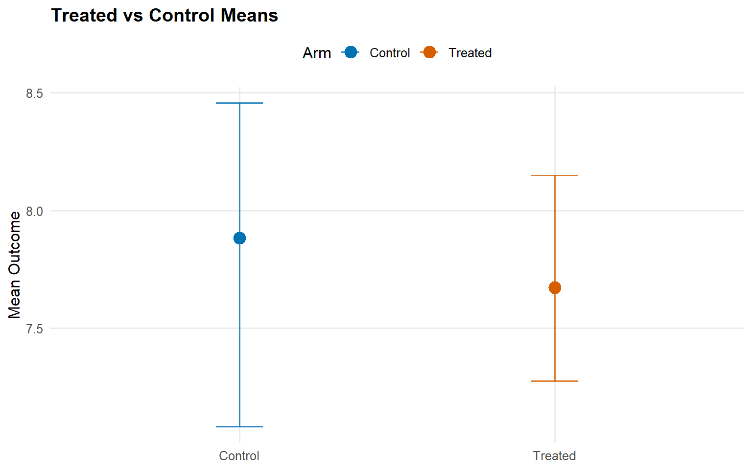
Code

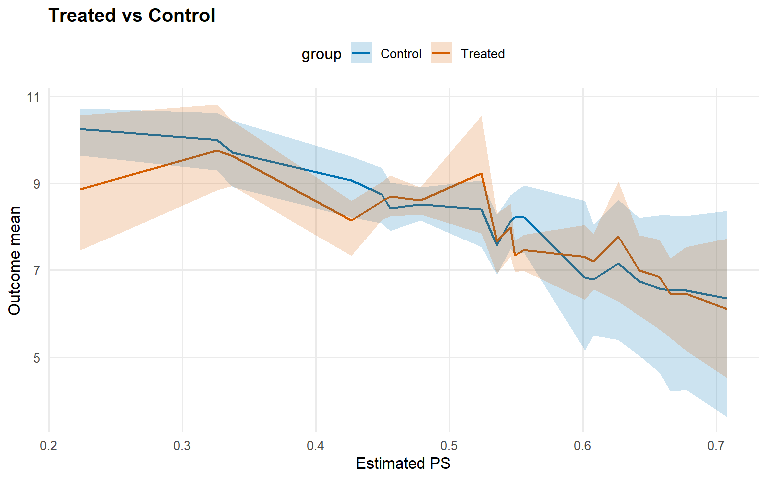
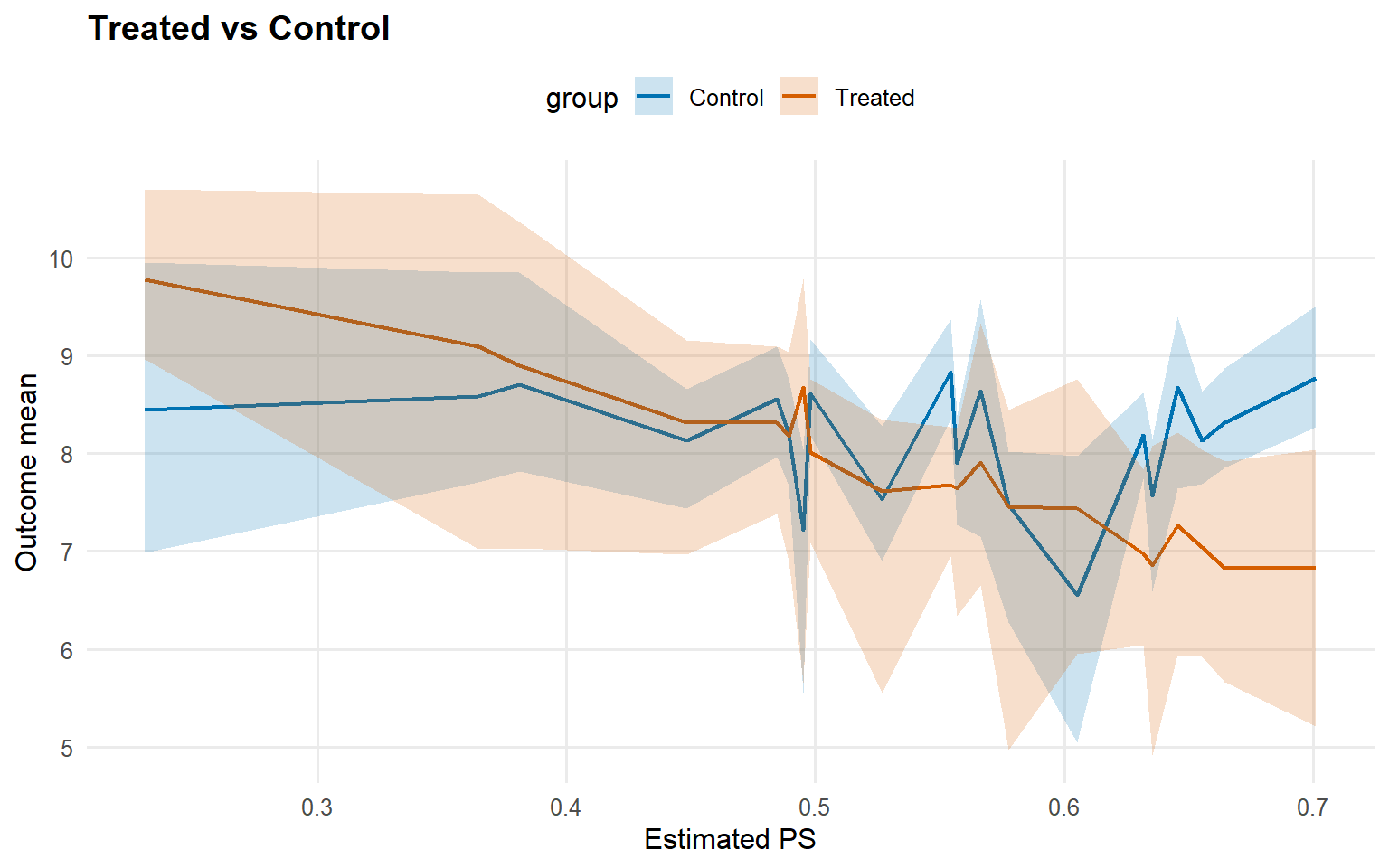
pred_mean_sb_crp <- predict(fit_sb_crp, newdata =x_eval, type = "mean",
                            interval = "credible", nsim_mean = nsim_mean_ex14, workers = predict_workers_ex14)
plot(pred_mean_sb_crp)

Code

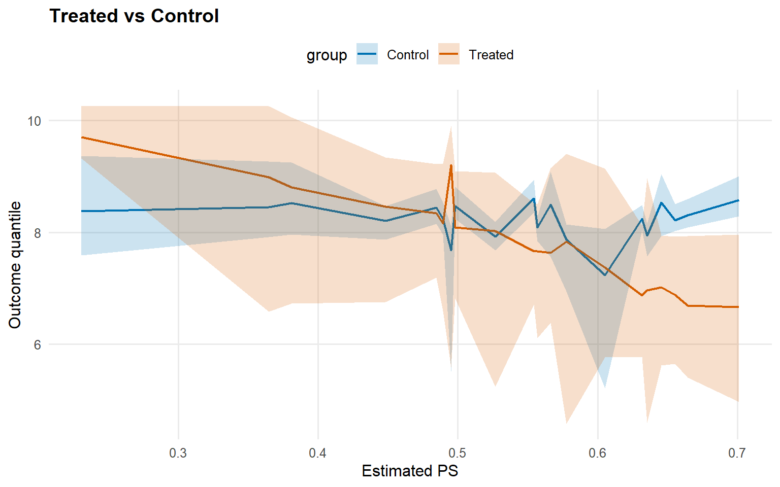
pred_q_sb_crp <- predict(fit_sb_crp, newdata =x_eval, type = "quantile",
                         p = 0.5, interval = "credible", workers = predict_workers_ex14)
plot(pred_q_sb_crp)

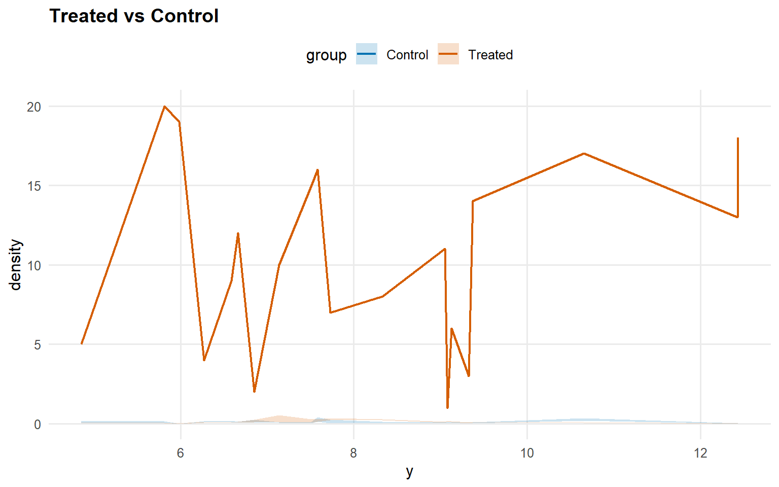
Code

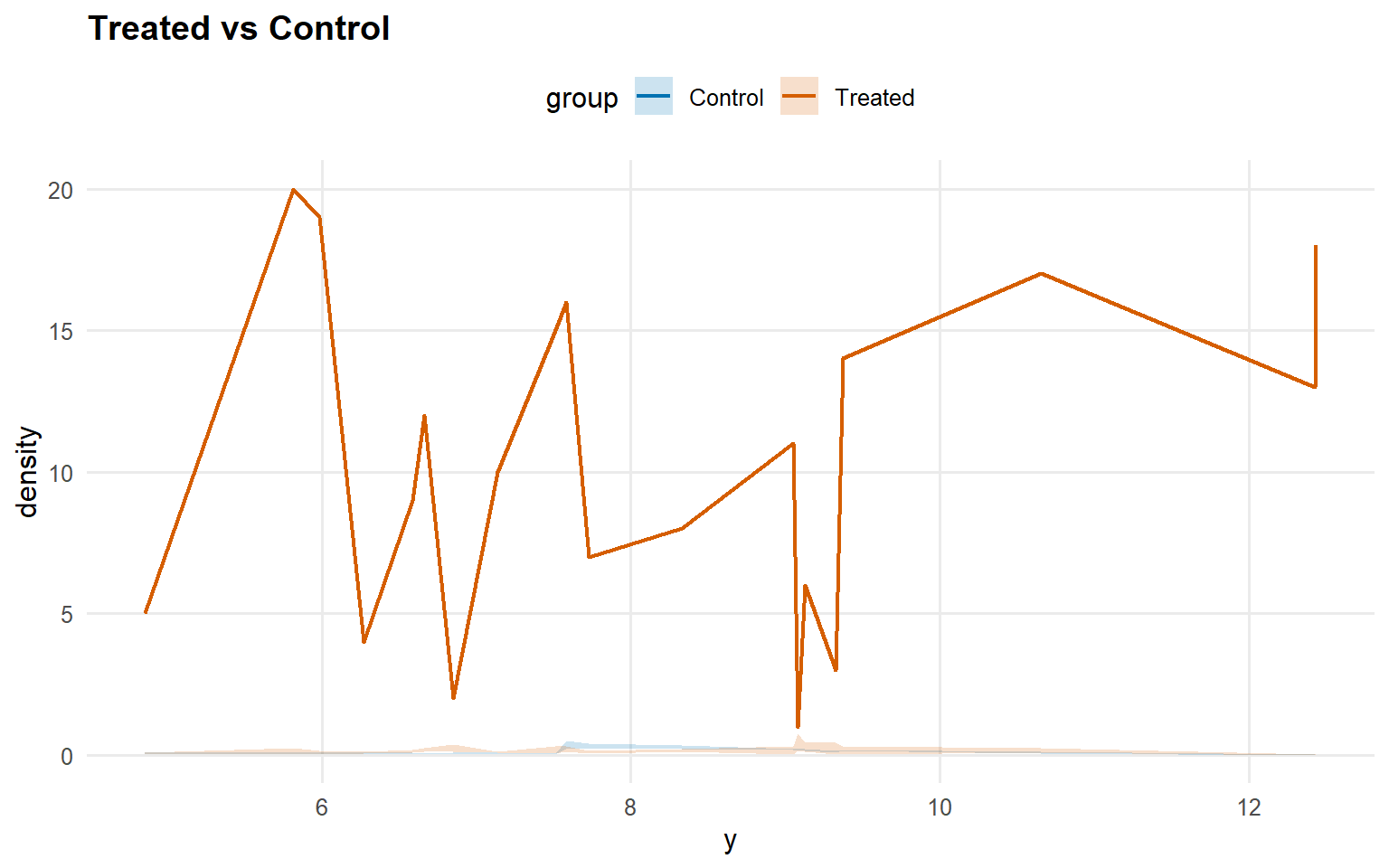
pred_d_sb_crp <- predict(fit_sb_crp, newdata =x_eval, y = y_eval,
                         type = "density", interval = "credible", workers = predict_workers_ex14)
plot(pred_d_sb_crp)

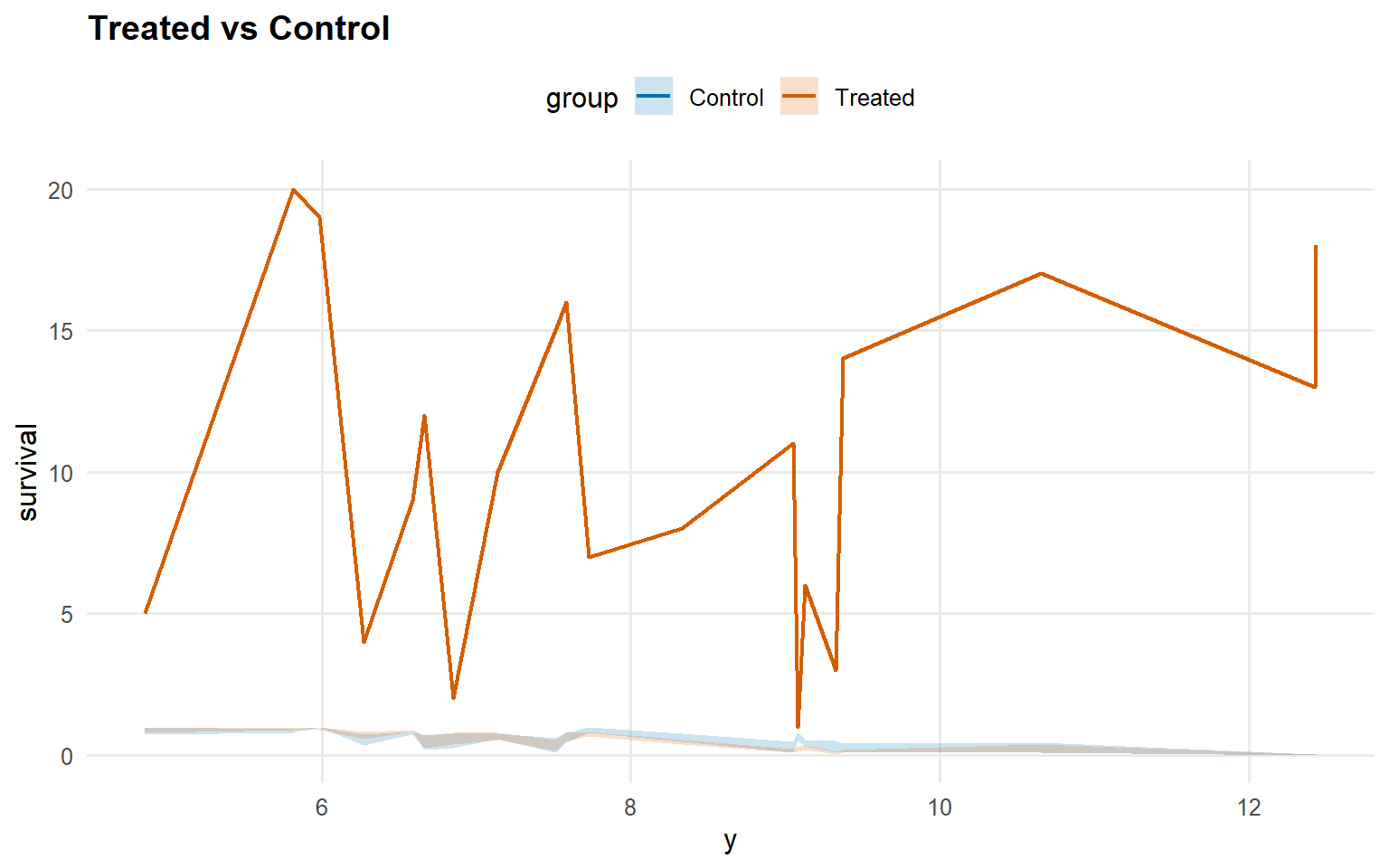
Code

pred_surv_sb_crp <- predict(fit_sb_crp, newdata =x_eval, y = y_eval,
                            type = "survival", interval = "credible", workers = predict_workers_ex14)
plot(pred_surv_sb_crp)

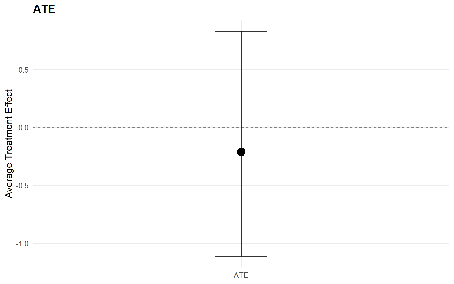
Code

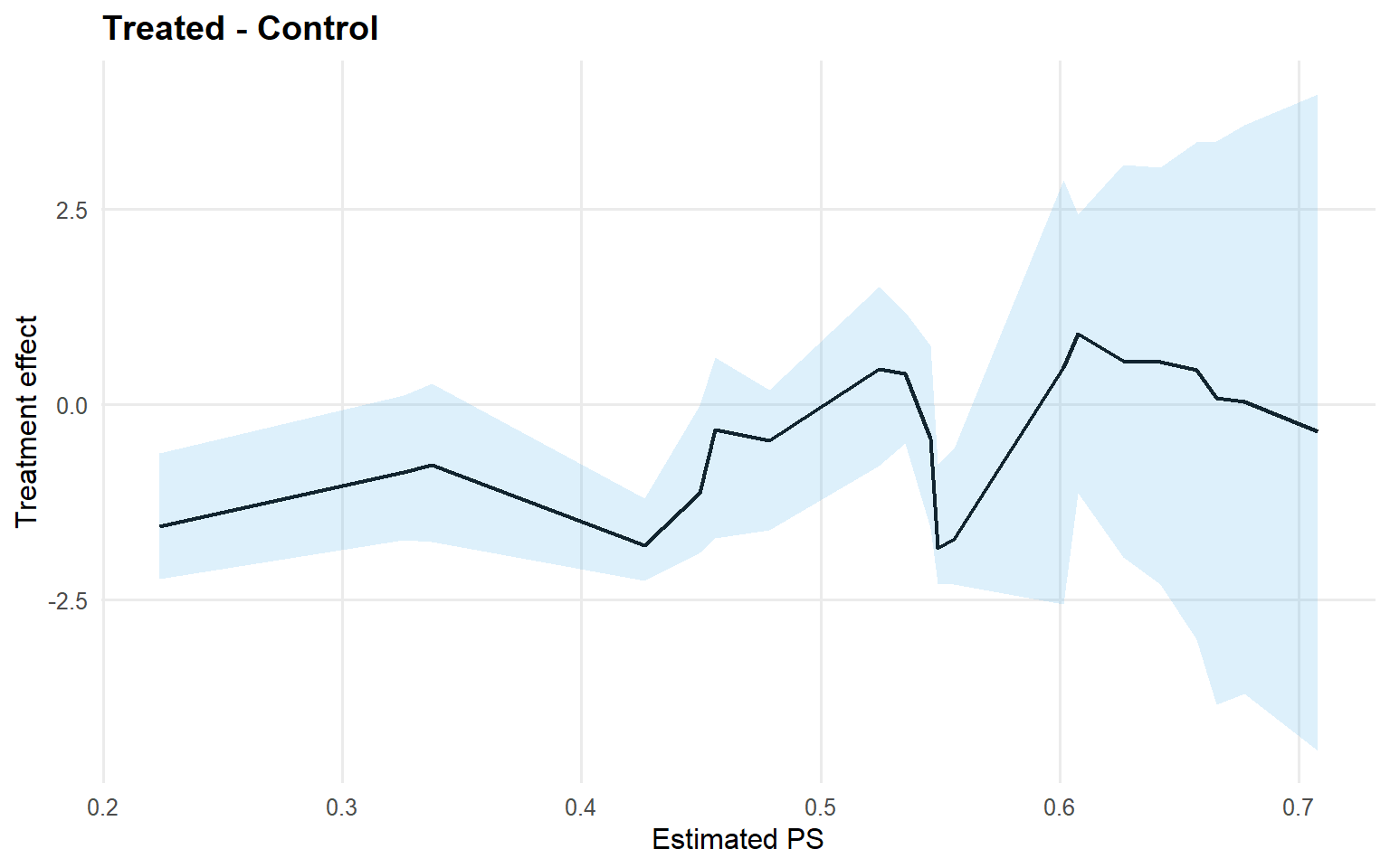
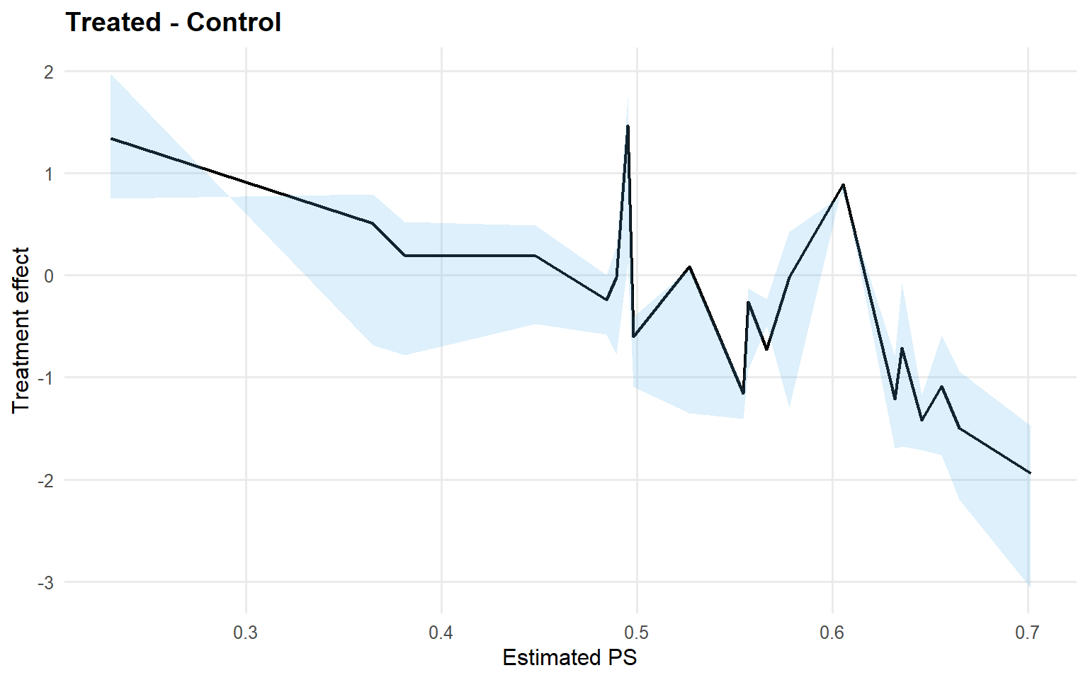
ate_sb_crp <- ate(fit_sb_crp, interval = "credible", nsim_mean = nsim_mean_ex14)
plot(ate_sb_crp)

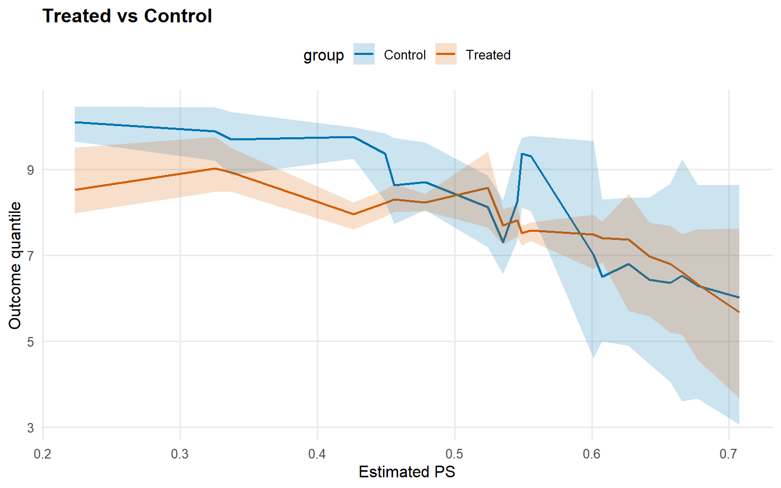
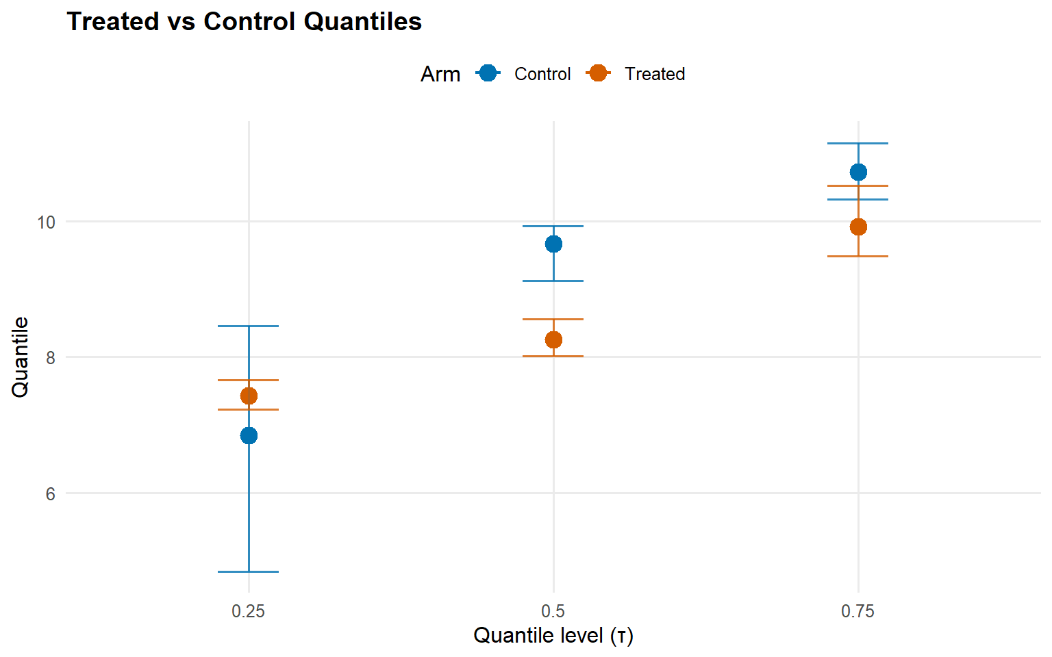
Code

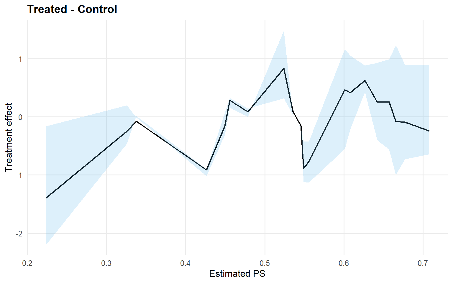
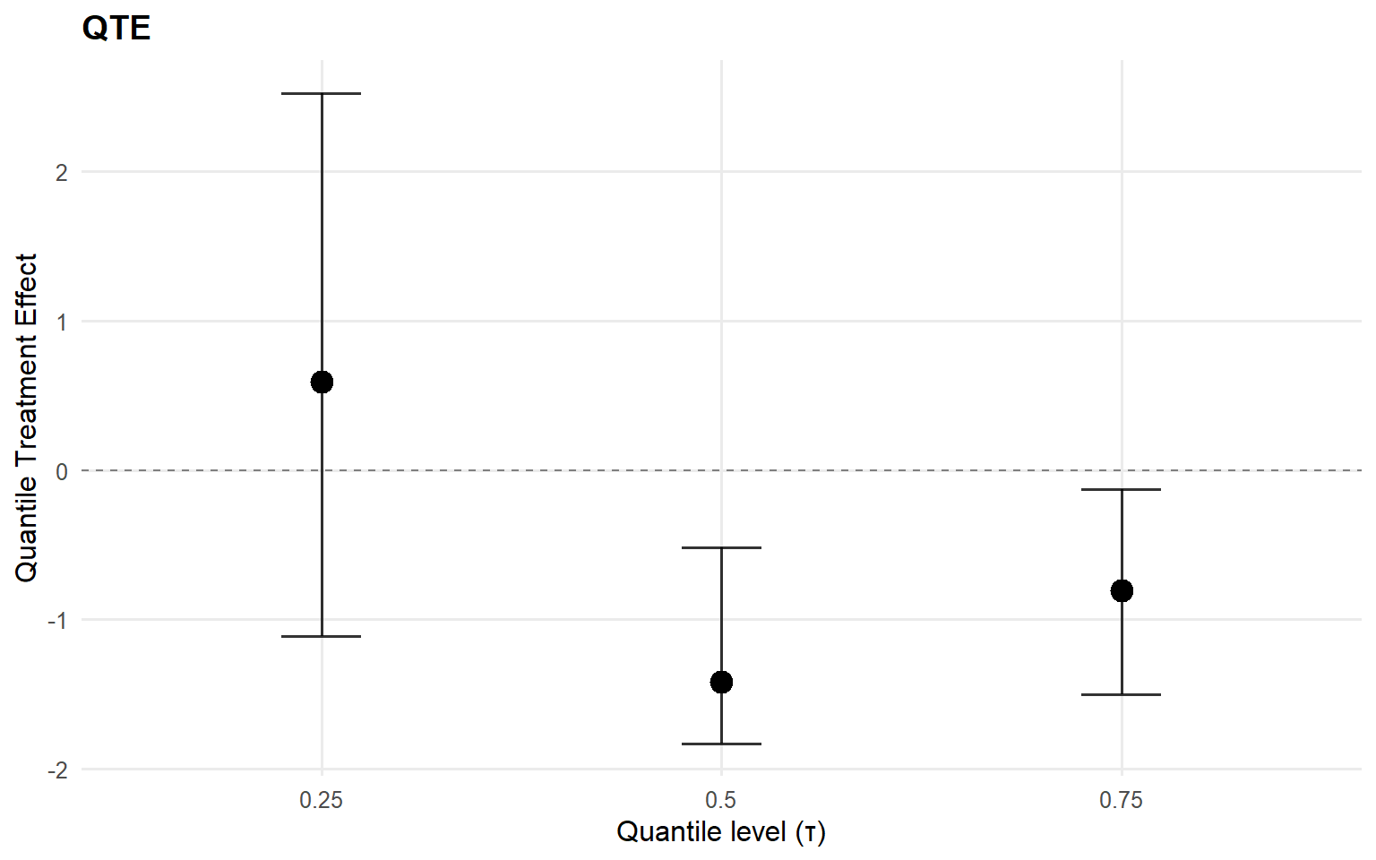
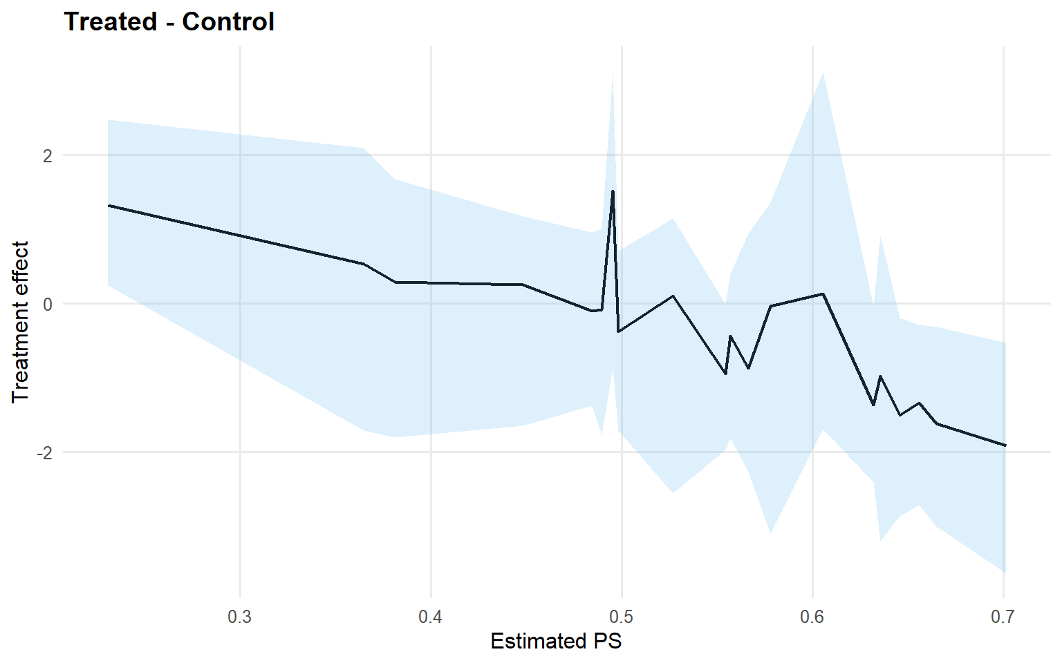
qte_sb_crp <- qte(fit_sb_crp, probs = c(0.25, 0.5, 0.75), interval = "credible")
plot(qte_sb_crp)

Model B: Treated CRP, Control SB (Amoroso + GPD)

Code

bundle_crp_sb <- bundle(
  y = y,
  treat = A,
  X = X,
  kernel = c("amoroso", "amoroso"),
  backend = c("crp", "sb"),
  PS = "logit",
  GPD = c(TRUE, TRUE),
  components = components_ex14,
  param_specs = param_specs_gpd,
  mcmc_outcome = gpd_mcmc_ex14_b,
  mcmc_ps = mcmc_ps_ex14_b
)

bundle_crp_sb

CausalMixGPD causal bundle
PS model: Bayesian logit (A | X) 
      Field                    Treated                Control
    Backend Chinese Restaurant Process Stick-Breaking Process
     Kernel                    amoroso                amoroso
 Components                          3                      3
   GPD tail                       TRUE                   TRUE
    Epsilon                      0.025                  0.025

Outcome PS included: TRUE 
n (control) = 232 | n (treated) = 268

Code

summary(bundle_crp_sb)

CausalMixGPD causal bundle summary
CausalMixGPD causal bundle
PS model: Bayesian logit (A | X) 
      Field                    Treated                Control
    Backend Chinese Restaurant Process Stick-Breaking Process
     Kernel                    amoroso                amoroso
 Components                          3                      3
   GPD tail                       TRUE                   TRUE
    Epsilon                      0.025                  0.025

Outcome PS included: TRUE 
n (control) = 232 | n (treated) = 268

Code

fit_crp_sb <- load_or_fit(
  tag_crp_sb_ex14,
  quiet_mcmc(dpmgpd.causal(bundle_crp_sb, mcmc = causal_run_mcmc))
)
summary(fit_crp_sb)

-- PS fit --
CausalMixGPD PS fit summary
model: logit 
n = 500 | predictors = 5
Monitors: beta 

Summary table
 parameter   mean    sd q0.025 q0.500 q0.975
   beta[1]  0.021 0.082 -0.056 -0.005  0.144
   beta[2]  0.458 0.082  0.324  0.451  0.607
   beta[3]   0.27 0.197 -0.042  0.216  0.544
   beta[4] -0.149 0.065 -0.303 -0.107  -0.07
   beta[5]  0.277 0.149 -0.228  0.348   0.48

-- Outcome fits --
[control]
MixGPD summary | backend: Stick-Breaking Process | kernel: Amoroso Distribution | GPD tail: TRUE | epsilon: 0.025
n = 232 | components = 3
Summary
Initial components: 3 | Components after truncation: 3

Summary table
          parameter   mean    sd q0.025 q0.500 q0.975
         weights[1]  0.493 0.014  0.487  0.487  0.527
         weights[2]  0.452  0.03  0.409  0.474  0.474
         weights[3]  0.055 0.023  0.038  0.038  0.099
              alpha  1.831 0.884  0.563  1.628  3.332
 beta_tail_scale[1] -0.053 0.056  -0.16 -0.052  0.052
 beta_tail_scale[2] -0.028 0.101 -0.185 -0.028   0.14
 beta_tail_scale[3] -0.045 0.049 -0.133  -0.04  0.033
 beta_tail_scale[4]  0.889 0.142   0.65  0.905  1.166
         tail_shape -0.077 0.022 -0.134 -0.084 -0.059
          threshold  7.544     0  7.544  7.544  7.544
          shape1[1]  5.107 0.924  4.032  4.943  7.146
          shape1[2]  7.159 1.559  5.078  7.293  9.654
          shape1[3]  2.642 1.475  0.238  2.694  5.982
          shape2[1]   0.47 0.071  0.382  0.508  0.536
          shape2[2]  0.985 0.028  0.955  0.971  1.016
          shape2[3]  1.119 1.165  0.131  0.495  3.515
      beta_loc[1,1]      0     0      0      0      0
      beta_loc[1,2]      0     0      0      0      0
      beta_loc[1,3]      0     0      0      0      0
      beta_loc[1,4]      0     0      0      0      0
      beta_loc[2,1]      0     0      0      0      0
      beta_loc[2,2]      0     0      0      0      0
      beta_loc[2,3]      0     0      0      0      0
      beta_loc[2,4]      0     0      0      0      0
      beta_loc[3,1]      0     0      0      0      0
      beta_loc[3,2]      0     0      0      0      0
      beta_loc[3,3]      0     0      0      0      0
      beta_loc[3,4]      0     0      0      0      0
    beta_scale[1,1] -0.263  0.47 -1.084 -0.277   0.76
    beta_scale[1,2]  0.429 0.735 -0.884  0.354  1.616
    beta_scale[1,3] -0.139 0.438 -0.795 -0.267   0.72
    beta_scale[1,4]  2.034 1.116  0.011  1.949  4.311
    beta_scale[2,1]  0.083 0.106  -0.15  0.072  0.259
    beta_scale[2,2]  0.051 0.107 -0.125  0.041   0.26
    beta_scale[2,3] -0.065 0.063 -0.194 -0.063  0.049
    beta_scale[2,4]  0.365 0.372 -0.275  0.254  0.993
    beta_scale[3,1] -0.287 2.184 -4.546 -0.539  4.407
    beta_scale[3,2] -0.271 2.018 -3.948 -0.152  3.665
    beta_scale[3,3] -0.127 1.554 -2.804 -0.451  3.516
    beta_scale[3,4]  1.636 2.272 -2.587  1.848  5.503

[treated]
MixGPD summary | backend: Chinese Restaurant Process | kernel: Amoroso Distribution | GPD tail: TRUE | epsilon: 0.025
n = 268 | components = 3
Summary
Initial components: 3 | Components after truncation: 1

WAIC: 100140.928
lppd: -501.379 | pWAIC: 49569.085

Summary table
          parameter   mean    sd q0.025 q0.500 q0.975
         weights[1]  0.841  0.17  0.567  0.918      1
              alpha  0.467  0.31  0.066  0.396  1.281
 beta_tail_scale[1]  0.043 0.079 -0.094  0.047   0.19
 beta_tail_scale[2] -0.153 0.121 -0.389 -0.144  0.088
 beta_tail_scale[3]  0.201 0.104  -0.02  0.204  0.398
 beta_tail_scale[4]  0.339 0.164  0.056  0.345  0.593
         tail_shape -0.104 0.026 -0.173 -0.102 -0.076
          threshold  9.028 0.072  9.003  9.003  9.292
          shape1[1]  6.772 0.785   4.73  7.022  7.499
          shape2[1]  0.875 0.018  0.861  0.861  0.908
      beta_loc[1,1]  0.566 1.416 -2.103  1.346  1.968
      beta_loc[1,2] -1.465 0.437 -2.125 -1.309 -0.617
      beta_loc[1,3] -0.953 0.237 -1.258 -0.838  -0.61
      beta_loc[1,4]  2.465 0.685   1.19  2.625  3.389
    beta_scale[1,1] -0.298 0.223  -0.61 -0.359   0.21
    beta_scale[1,2]   0.15 0.159 -0.151  0.186  0.448
    beta_scale[1,3]  0.216 0.052  0.133  0.213  0.327
    beta_scale[1,4] -0.528 0.234 -0.866 -0.558   0.05

Code

params(fit_crp_sb)

Posterior mean parameters (causal)

[ps]
Posterior mean parameters

$beta
[1]  0.02086  0.45850  0.27050 -0.14870  0.27740

[treated]
Posterior mean parameters

$alpha
[1] 0.4674

$w
[1] 0.8415

$beta_loc
      PropScore    x1     x2      x3    x4
comp1    0.8991 0.566 -1.465 -0.9532 2.465

$beta_scale
      PropScore      x1     x2     x3      x4
comp1    0.3048 -0.2978 0.1501 0.2158 -0.5283

$shape1
[1] 6.772

$shape2
[1] 0.8754

$threshold
[1] 9.028

$beta_tail_scale
             x1      x2     x3     x4
overall 0.04303 -0.1532 0.2008 0.3389

$tail_shape
[1] -0.1039

[control]
Posterior mean parameters

$alpha
[1] 1.831

$w
[1] 0.49320 0.45200 0.05482

$beta_loc
      PropScore x1 x2 x3 x4
comp1         0  0  0  0  0
comp2         0  0  0  0  0
comp3         0  0  0  0  0

$beta_scale
      PropScore       x1      x2       x3     x4
comp1   0.38570 -0.26260  0.4291 -0.13890 2.0340
comp2  -0.27440  0.08262  0.0505 -0.06538 0.3653
comp3  -0.02691 -0.28680 -0.2711 -0.12710 1.6360

$shape1
[1] 5.107 7.159 2.642

$shape2
[1] 0.4696 0.9845 1.1190

$threshold
[1] 7.544

$beta_tail_scale
              x1       x2       x3     x4
overall -0.05256 -0.02801 -0.04545 0.8895

$tail_shape
[1] -0.07651

Code

plot(fit_crp_sb, family = plot_family_crp_sb_ex14)


=== treated ===

=== density ===


=== control ===

=== density ===

Code

pred_mean_crp_sb <- predict(fit_crp_sb, newdata =x_eval, type = "mean",
                            interval = "credible", nsim_mean = nsim_mean_ex14, workers = predict_workers_ex14)
plot(pred_mean_crp_sb)

Code

pred_q_crp_sb <- predict(fit_crp_sb, newdata =x_eval, type = "quantile",
                         p = 0.5, interval = "credible", workers = predict_workers_ex14)
plot(pred_q_crp_sb)

Code

pred_d_crp_sb <- predict(fit_crp_sb, newdata =x_eval, y = y_eval,
                         type = "density", interval = "credible", workers = predict_workers_ex14)
plot(pred_d_crp_sb)

Code

pred_surv_crp_sb <- predict(fit_crp_sb, newdata =x_eval, y = y_eval,
                            type = "survival", interval = "credible", workers = predict_workers_ex14)
plot(pred_surv_crp_sb)

Code

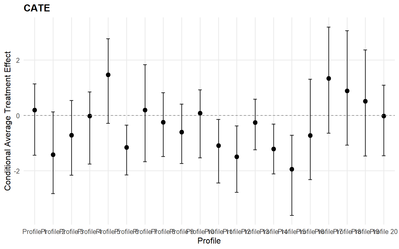
cate_crp_sb <- cate(fit_crp_sb, newdata = x_eval,
                   interval = "credible", nsim_mean = nsim_mean_ex14)
head(format_cate_table(cate_crp_sb))

  id index    estimate      lower      upper
1  1     1  0.18953974 -1.4347426  1.1397729
2  2     1 -1.41838105 -2.8257883  0.1279135
3  3     1 -0.71391510 -2.1527255  0.5422384
4  4     1 -0.02181351 -1.7503993  0.8510921
5  5     1  1.46568595 -0.2840095  2.7674652
6  6     1 -1.15685357 -2.1452202 -0.3455291

Code

plot(cate_crp_sb)

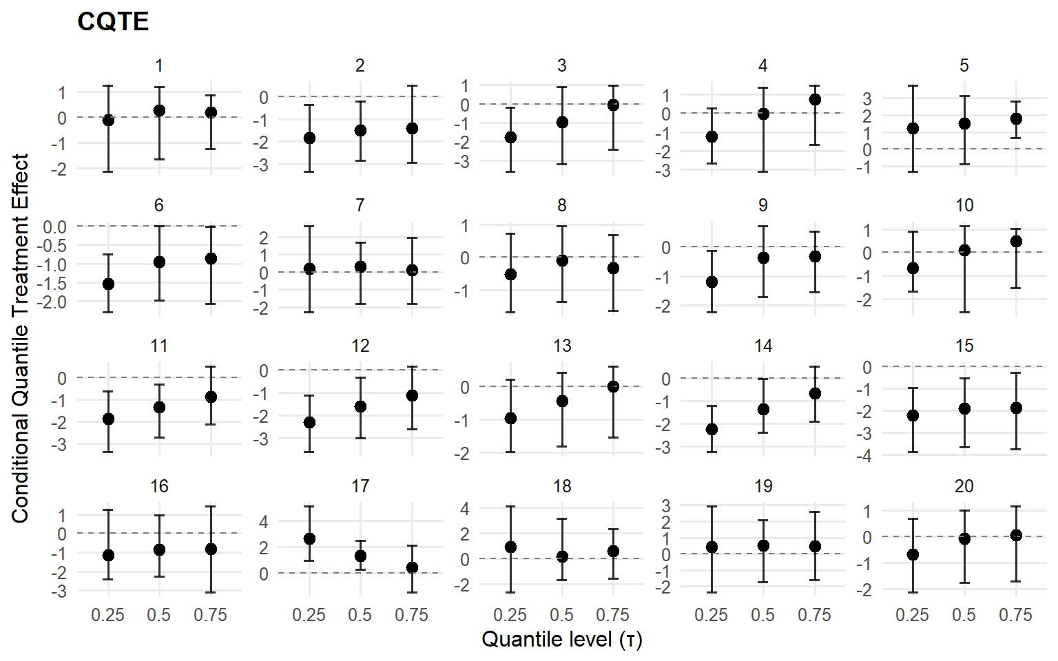
Code

cqte_crp_sb <- cqte(fit_crp_sb, probs = c(0.25, 0.5, 0.75),
                   newdata = x_eval, interval = "credible")
head(format_cqte_table(cqte_crp_sb))

  id index   estimate     lower      upper
1  1     1 -0.1229123 -2.135624  1.2259354
2  1     2  0.2534521 -1.649174  1.1700091
3  1     3  0.1790422 -1.239670  0.8398795
4  2     1 -1.8316943 -3.343504 -0.3658125
5  2     2 -1.5103598 -2.865960 -0.1963388
6  2     3 -1.4044933 -2.934697  0.5036670

Code

plot(cqte_crp_sb)

Prereqs

Required packages and data for this page are listed in the setup chunks above.

Outputs

This page renders model fits, diagnostics, and summary artifacts generated by package APIs.

Interpretation

Canonical concept page: 03 Causal Inference Objects
Treat this page as an application/example view and use the canonical page for core definitions.

Continue to the linked canonical concept page, then return for implementation-specific details.

ex14. Causal (Different backends, SB Backend) - Amoroso Kernel

Causal Inference: Mixed Backends with GPD - Amoroso Kernel

What you’ll learn

Compare against the bulk-only mixed-backend setup to isolate the incremental impact of `GPD = TRUE`.

Data Setup

Model A: Treated SB, Control CRP (Amoroso + GPD)

Model B: Treated CRP, Control SB (Amoroso + GPD)

Workflow Navigation

Prereqs

Outputs

Interpretation

Next

Causal Inference: Mixed Backends with GPD - Amoroso Kernel

What you’ll learn

Compare against the bulk-only mixed-backend setup to isolate the incremental impact of GPD = TRUE.

Data Setup

Model A: Treated SB, Control CRP (Amoroso + GPD)

Model B: Treated CRP, Control SB (Amoroso + GPD)

Workflow Navigation

Prereqs

Outputs

Interpretation

Next

Compare against the bulk-only mixed-backend setup to isolate the incremental impact of `GPD = TRUE`.