ex15. Clustering with GPD Tail (Weights + Covariates)

Website workflow note. This page reflects the current exported clustering API built around dpmgpd.cluster(), predict(), summary(), and plot(). Last updated: 2026-03-19.

For the package-level theory and longer narrative, see the manuscript and the clustering discussion in the main package articles.

Clustering with a Spliced GPD Tail and Covariate-Dependent Weights

What you’ll learn

How to fit tail-aware clustering with dpmgpd.cluster().
How the type = "weights" dependence mode uses covariates to change cluster prevalence (mixture weights), while keeping component likelihood structure shared.
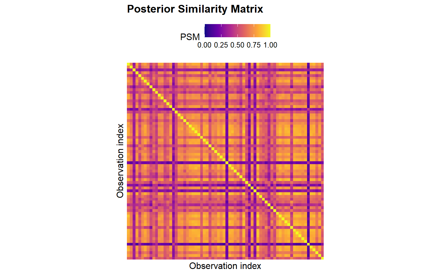
How to use predict() to obtain labels and a posterior similarity matrix (PSM), and how to interpret the label/PSM plots.

Purpose (in one sentence)

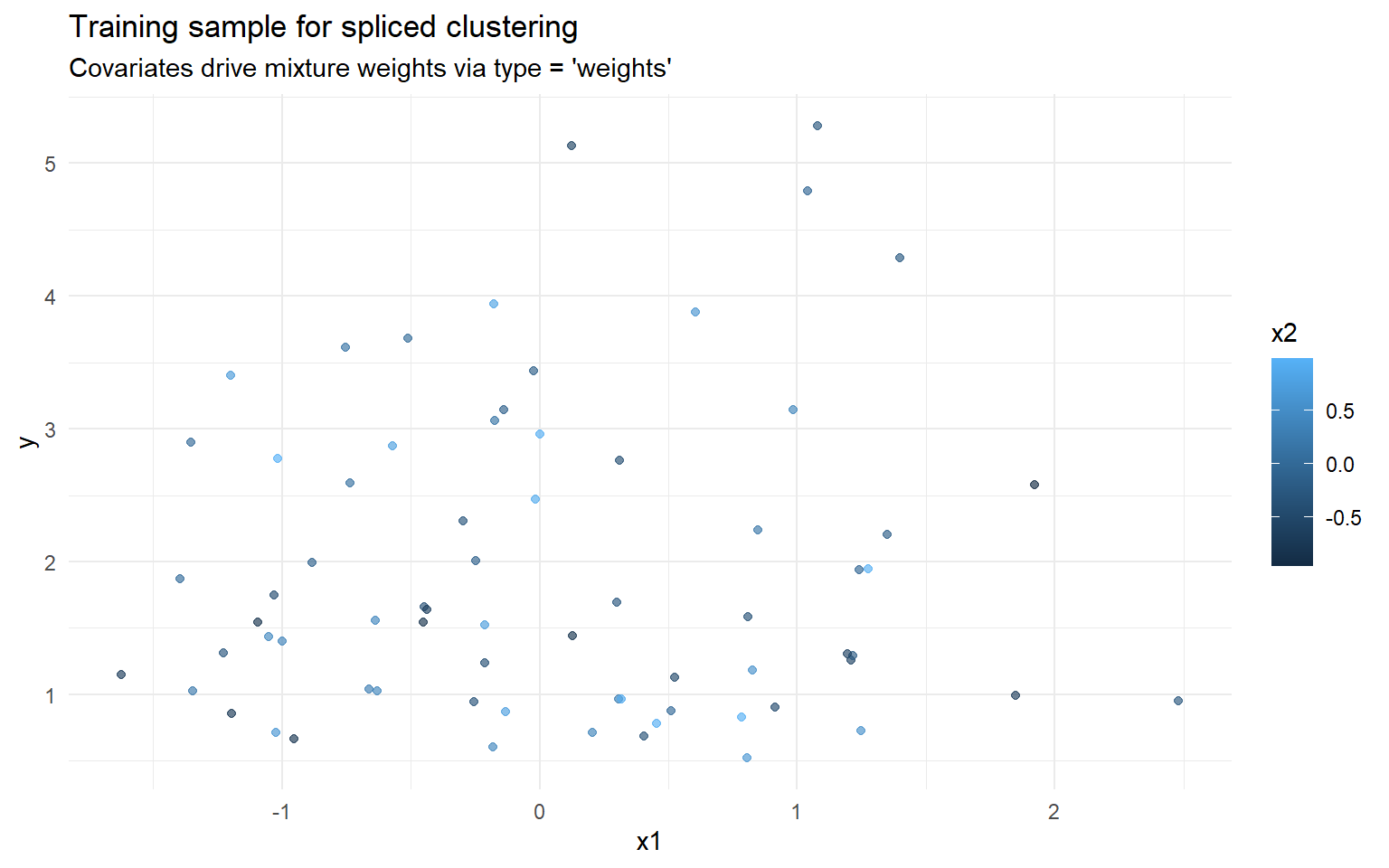
Fit a tail-aware clustering model where covariates affect cluster prevalence through mixture weights (type = "weights"), and the component likelihood is a spliced bulk + GPD tail model.

Data Setup

Code

data("nc_posX100_p5_k4")
dat <- data.frame(y = nc_posX100_p5_k4$y, nc_posX100_p5_k4$X)

train_id <- seq_len(70)
train_dat <- dat[train_id, , drop = FALSE]
test_dat <- dat[-train_id, , drop = FALSE]

summary_tbl <- tibble(
  split = c("train", "test"),
  n = c(nrow(train_dat), nrow(test_dat)),
  y_mean = c(mean(train_dat$y), mean(test_dat$y)),
  y_sd = c(stats::sd(train_dat$y), stats::sd(test_dat$y)),
  y_max = c(max(train_dat$y), max(test_dat$y))
)

summary_tbl

# A tibble: 2 × 5
  split     n y_mean  y_sd y_max
  <chr> <int>  <dbl> <dbl> <dbl>
1 train    70   1.94  1.17  5.28
2 test     30   1.96  1.11  4.18

Code

ggplot(train_dat, aes(x = x1, y = y, color = x2)) +
  geom_point(alpha = 0.65) +
  labs(
    title = "Training sample for spliced clustering",
    subtitle = "Covariates drive mixture weights via type = 'weights'",
    x = "x1",
    y = "y",
    color = "x2"
  ) +
  theme_minimal()

Fit a Spliced Clustering Model

Code

fit_cluster_gpd <- load_or_fit(
  "ex15-clustering-dpmgpd-weights-fit_cluster_gpd",
  dpmgpd.cluster(
    y ~ x1 + x2 + x3 + x4 + x5,
    data = train_dat,
    kernel = "lognormal",
    type = "weights",
    components = 10,
    mcmc = mcmc
  )
)

summary(fit_cluster_gpd, vars = c("y", "x1", "x2", "x3"))

$K_star
[1] 5

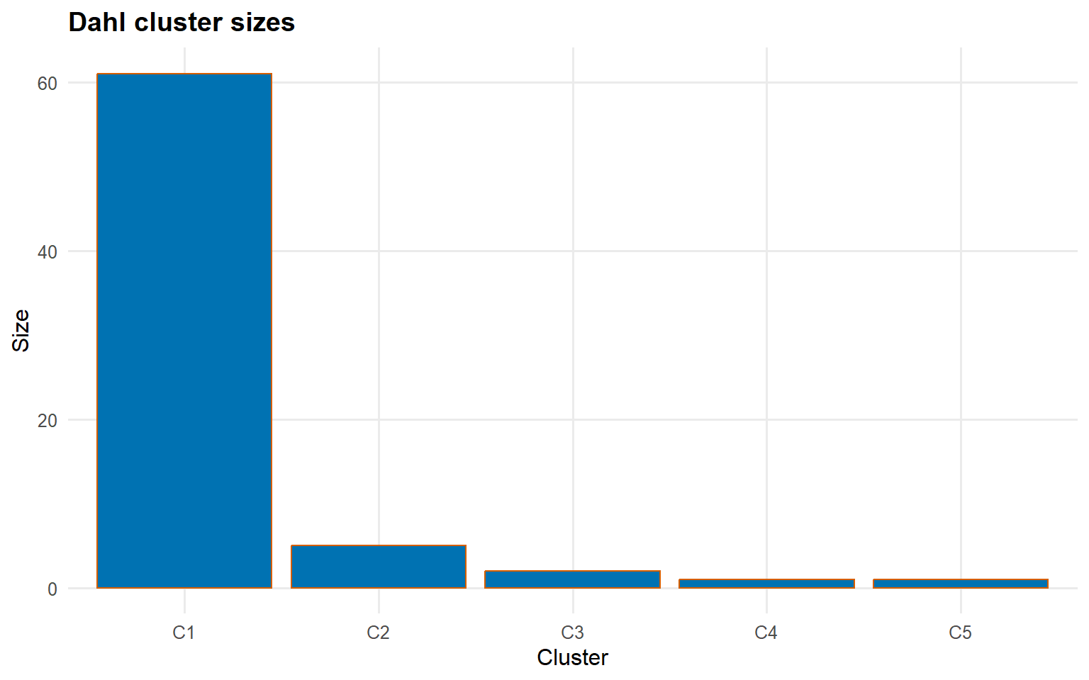
$cluster_sizes

 1  2  3  4  5 
61  5  2  1  1 

$cluster_profiles
  cluster  n    y_mean      y_sd      x1_mean     x1_sd     x2_mean     x2_sd
1      C1 61 1.9519186 1.1309051 -0.008098264 0.9277559  0.04763821 0.5634605
2      C2  5 1.5332865 0.8451246  0.465058447 0.8558037  0.17916220 0.3363054
3      C3  2 0.7717176 0.1199999 -0.395431116 1.1312839 -0.55624407 0.2742523
4      C4  1 1.9395389        NA  1.241187447        NA -0.04143591        NA
5      C5  1 5.2783434        NA  1.079272215        NA -0.28493860        NA
     x3_mean     x3_sd certainty_mean certainty_sd
1 -0.0217340 0.9401597      0.3124220   0.03614309
2 -0.3689271 1.0437381      0.2656916   0.02948265
3  0.9168566 0.5688655      0.3065634   0.01406759
4  1.2865362        NA      0.3995354           NA
5 -0.8084690        NA      0.4036634           NA

$certainty
   Min. 1st Qu.  Median    Mean 3rd Qu.    Max. 
 0.2209  0.2919  0.3205  0.3115  0.3383  0.4037 

$source
[1] "train"

$burnin
[1] 0

$thin
[1] 1

attr(,"class")
[1] "summary.dpmixgpd_cluster_fit" "list"

This clustering configuration uses the formula/data-frame interface directly. Because type = "weights", covariates enter the gating model for cluster membership, while the spliced bulk-tail likelihood captures upper-tail differences inside each component.

Training Labels and Posterior Similarity Matrix

Code

cluster_psm_gpd <- predict(fit_cluster_gpd, type = "psm")
cluster_train_gpd <- predict(fit_cluster_gpd, type = "label", return_scores = TRUE)

train_summary_gpd <- summary(
  cluster_train_gpd,
  vars = c("y", "x1", "x2", "x3"),
  top_n = 5
)

train_sizes_tbl <- tibble(
  cluster = paste0("C", names(train_summary_gpd$cluster_sizes)),
  n = as.integer(train_summary_gpd$cluster_sizes)
)

train_sizes_tbl

# A tibble: 5 × 2
  cluster     n
  <chr>   <int>
1 C1         61
2 C2          5
3 C3          2
4 C4          1
5 C5          1

Code

plot(cluster_psm_gpd)

Code

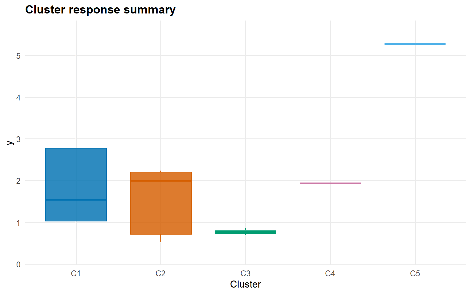
plot(cluster_train_gpd, type = "summary", top_n = 5)

The PSM summarizes posterior co-clustering probabilities on the training sample, while the training label object gives the Dahl representative partition together with assignment scores and cluster-level summaries.

Predict Labels for New Observations

Code

cluster_new_gpd <- predict(
  fit_cluster_gpd,
  newdata = test_dat,
  type = "label",
  return_scores = TRUE
)

new_summary_gpd <- summary(
  cluster_new_gpd,
  vars = c("y", "x1", "x2", "x3"),
  top_n = 5
)

new_sizes_tbl <- tibble(
  cluster = paste0("C", names(new_summary_gpd$cluster_sizes)),
  n = as.integer(new_summary_gpd$cluster_sizes)
)

new_sizes_tbl

# A tibble: 1 × 2
  cluster     n
  <chr>   <int>
1 C1         30

Code

plot(cluster_new_gpd, type = "certainty")

Code

plot(fit_cluster_gpd, which = "sizes", top_n = 5)

predict(..., newdata = ..., type = "label") maps held-out observations into the space of the representative training clusters. The returned score matrix can be summarized either numerically or with the built-in certainty plot above.

Takeaways

dpmgpd.cluster() is the current wrapper for tail-aware clustering.
type = "weights" is appropriate when covariates should change cluster prevalence rather than cluster-specific kernel parameters.
The standard post-fit workflow is predict(..., type = "psm"), predict(..., type = "label"), then summary()/plot() on the returned cluster objects.
The next page contrasts this with a bulk-only clustering model where covariates enter through parameter links instead of weights.

Prereqs

Required packages and data for this page are listed in the setup chunks above.

Outputs

This page renders model fits, diagnostics, and summary artifacts generated by package APIs.

Interpretation

Canonical concept page: 02 Clustering Extension
Treat this page as an application/example view and use the canonical page for core definitions.

Continue to the linked canonical concept page, then return for implementation-specific details.

ex15. Clustering with GPD Tail (Weights + Covariates)

Clustering with a Spliced GPD Tail and Covariate-Dependent Weights

What you’ll learn

Purpose (in one sentence)

Data Setup

Fit a Spliced Clustering Model

Training Labels and Posterior Similarity Matrix

Predict Labels for New Observations

Takeaways

Workflow Navigation

Prereqs

Outputs

Interpretation

Next